Stochastic versus Deterministic Approaches - Environmental Modelling: Finding Simplicity in Complexity - page 142

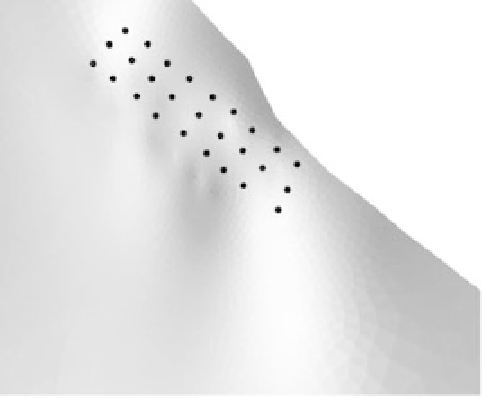
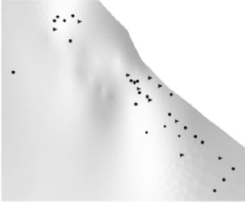
(a) (b)

1

1

Optimal
Min: 4.7
Mean: 9.5
Max: 14.7

Optimal
Min: 8.7
Mean: 9.2
Max: 9.9

0.8

0.8

Synthetic
Min: 7.7
Mean: 17.1
Max: 37.0

0.6

0.6

0.4

0.4

Synthetic
Min: 9.6
Mean: 9.2
Max: 10.0

0.2 0.2

0 0

8.4 8.8 9.2 9.6

Cost [Million Euros]

10 10.4 0 10 20 30

Hydraulic head at pumping well [m]

40

(c) (d)

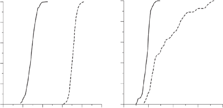
Figure 8.8 Synthetic (a) and optimum (b) pumping networks. Pumping rates of 100 l s − 1 ,70ls − 1 and 30 l s − 1 are depicted with
circles, triangles and squares, respectively. On the background, the average transmissivity field plotted with the same scale as in
Figure 8.6. Cumulative distribution functions of optimal (solid line) and synthetic (dashed line) pumping networks: (c) cost
function, (d) hydraulic head drop at pumping wells.

describing the internal (molecule to molecule) complex-
ity. In that upscaling process, we see through the use
of stochastic methods the emergence of different levels
of deterministic laws. A second example that has been
used here to illustrate different concepts is groundwa-
ter flow, which can be described by the Navier-Stokes
equations if the three dimensional geometry of the pore

network is known and if one can discretize the pore space
finely. That approach is indeed limited to very small
samples of material (a few mm 3 ) to be amenable to solu-
tion with existing computers. However, one can define
expected values for the pressure (or hydraulic head) and
the fluid velocities and derive analytical expressions for
the mean behaviour of the fluid on a larger domain.