Environmental Engineering Reference
In-Depth Information
7
2
E[h]
E[h]
+
/
−
2
σ
h(p
max
,r
max
), h(p
min
,r
min
)
6
1.5
5
4
1
3
2
0.5
1
0
0
0
1000
2000 3000
distance to river [m]
4000
5000
2
2.5
3
3.5
h(x = 2000)
4
4.5
5
(a)
(b)
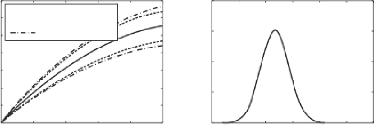
Figure 8.3
(a) Comparison between uncertainties obtained by deterministic and stochastic models. Recharge is the only uncertain
parameter. In black, expected head distribution along the flow line obtained by the stochastic model (visually comparable to that in
Figure 8.2b, output of the deterministic model). The uncertainty is estimated either using the stochastic approach of Equation (8.13)
(inner dashed lines), or using a min/max deterministic approach (outer dashed lines); (b) probability density function of hydraulic
head at the location of the building obtained by using Equation (8.13) and the assumption of Gaussian uncertainty.
either through small perturbation analysis, in which the
variables are decomposed as a mean plus a perturbation
around it. By construction, this perturbation has a zero
mean, and a variance equal to the variance of the original
variable. Plugging these definitions into the deterministic
equation, one obtains an equation that is then decom-
posed into subquations of same order. To solve it, one can
neglect terms that are considered of small order and obtain
approximate solutions. A simple illustrative example can
be found in de Marsily (1989). In the field of groundwater
hydrology, one can find a detailed description of those
techniques as well as a recent overview of the main results
in the topics by Zhang (2002) or Rubin (2003).
However, the limitation of the perturbation approach
and other approximate techniques is that their results
are valid only for small variances. In addition, the results
are usually expressed in terms of mean, variance and
covariance even if the distribution is known to be non-
multi-Gaussian (for example, the variance does not need
to be bounded). To overcome these limitations, the most
general approach is the Monte Carlo method (Metropolis
and Ulam, 1949). It generates a series of samples from
the statistical distribution of the input parameters and
solves the deterministic equations (either analytically or
numerically) for each set of parameters. One then obtains
an ensemble of responses for the variable of interest.
Repeating the operation a large number of times (sam-
pling the parameter space exhaustively) allows us to infer
the statistics of the variable of interest.
To illustrate how this method works and to demon-
strate the importance of such analysis, we will consider
again the groundwater problem of Figure 8.2. However,
this time we will consider that the hydraulic conduc-
tivity varies in space and, indeed, that it is not known
everywhere in the domain. We will assume just that the
hydraulic conductivity follows a log-normal distribution
with known mean
k
10
−
2
ms
−
1
2
1,.
This might seem a strong assumption. However, normal-
ity is often supported by field data (or a suitable transform
of them, as logarithmic in this case). We will also assume
that the log-hydraulic conductivity field can be modelled
by a multi-Gaussian spatially correlated field having an
exponential covariance function with a correlation range
of 200 m. Figure 8.4a displays an example of a corre-
lated random field generated with those parameters. The
hydraulic conductivity is centred on the value used pre-
viously in the deterministic model (
k
=
and variance
σ
ln
=
10
−
2
ms
−
1
)and
varies within an order of magnitude around this mean
value. This field is not conditioned to any local data. We
have generated 2000 hydraulic conductivity fields for the
Monte Carlo analysis. They all look similar but vary in
a random manner around the mean with structures that
always display the same pattern type and size. For each
field, Equation (8.10) is solved numerically by integrating
the hydraulic head along the flow line. This provides 2000
equally likely distributions. Two of them are depicted as
dashed lines in Figure 8.4c. These are comparable with
the deterministic analytical solution depicted as a dashed
lines in Figure 8.4b. The first observation that becomes
apparent from Figure 8.4c is the effect of the heterogeneity
of
k
, translated into local variations of the slope of the
dashed curves.
=


Search WWH ::

Custom Search