Environmental Engineering Reference
In-Depth Information
7.8.1 EmulationoftheHEC-RASRiverFlowModel
where
z
−
1
is the backward shift operator, i.e.
z
−
1
y
k
=
y
k
−
1
, so that the model can be written alternatively in the
discrete-time difference equation form:
y
j
,
k
=−
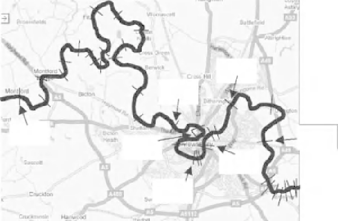
In this example, the large and complex HEC-RAS model is
a distributed parameter representation of flow in the River
Severn formed from 89 cross-sectional nodes between
Montford and Buildwas, as shown in Figure 7.8. The HEC-
RAS model solves the dynamic, Saint-Venant equations
using an implicit, finite difference method based on the
Preissman scheme. This model is run in an unsteady
flow mode and forced with an upstream boundary condi-
tion defined by uniformly sampled observations of flow
at Montford between December and March 2002, with
a sampling interval
6
(7.9)
Here, the function
f
j
(
y
j
,
k
−
1
) is an SDP nonlinearity
which is a function of the measured (here simulated)
y
j
,
k
−
1
and acts as a time-variable gain on the delayed
input variable
u
k
,
δ
j
. The estimated parameters of this
model are shown in Table 7.1, in which
T
j
is the residence
time in hours derived from the estimated parameter
a
j
,1
by the relationship
T
j
=−
1
/
log
e
(
−
a
j
,1
). The estimated
SDP input nonlinearities are shown in Figure 7.9.
This nominal emulation model explains the data well,
with coefficients of determination of
R
T
>
0
a
j
,1
y
j
,
k
−
1
+
b
j
,0
f
j
(
y
j
,
k
−
1
)
u
k
−
δ
j
j
=
1, 2,
···
t
of one hour. This observation
period contains a number of high-flow events resulting in
maximum simulated flows in Shrewsbury of 213 m
3
s
−
1
.
The maximum flows generate over-bank inundation at
all but six of the 89 nodes. The water-surface-level field
generated by the unsteady simulation run of HEC-RAS is
used as the estimation data set for the nominal emulation
model in the DME modelling exercise. For validation
purposes, two further simulations are carried out using
different input-level sequences.
Since the HEC-RAS model is simulated in the form of
finite difference equations, the DBM emulation model for
six of the cross-sections is also identified and estimated
in a discrete-time form using the RIVBJ algorithm in
CAPTAIN. The resulting model is remarkably simple and
takes the form of six first-order discrete-time transfer
functions with a sampling interval of one hour:
99 for each
of the six chosen cross-sections. More importantly, the
explanation is quite similar in the case of the validation
exercises, where a completely new input series is used to
drive the HEC-RAS model: the DME model outputs in
these validation exercises are compared with the HEC-
RAS model outputs in Figure 7.10, where the confidence
intervals are so small they are hardly visible.
In order to convert the model (7.8) to a full DME, it is
necessary to develop the parametric mapping, as indicated
in Figure 7.7, between specified HEC-RAS model param-
eters and the minimal order DME model parameters. For
simplicity, the input SDP nonlinearities obtained in the
nominal emulation model estimation were maintained
for the full DME model identification, so that the only
DME parameters that had to be re-estimated, at each real-
ization, using the RIVBJ algorithm were the two, linear
.
b
j
,0
y
j
,
k
=
a
j
,1
z
−
1
f
j
(
y
j
,
k
−
1
)
u
k
−
δ
j
j
=
1, 2,
···
6
(7.8)
1
+
cs 70
cs 82
input
cs 68
cs 79
cs 73
cs 77
Figure 7.8
The section of River Severn
Modelled by HEC-RAS (
2009
Google-Map data
2009 Google).


Search WWH ::

Custom Search