Environmental Engineering Reference
In-Depth Information
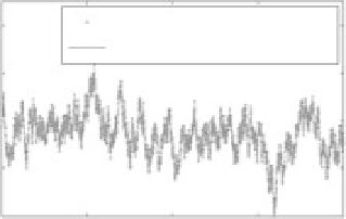
Layer 1 (R
T
= 0.999)
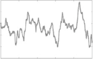
Layer 4 (R
T
= 0.999)
0.1
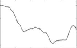
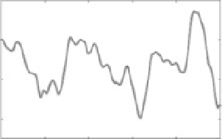
Large model output
Emulation model output
0.4
0.05
0.2
0
0
−
0.05
−
0.2
−
0.1
−
0.4
0
50
100
150
200
0
200
400
Time (years)
600
800
Time (years)
Layer 8 (R
T
= 0.999)
Layer 16 (R
T
= 0.999)
x 10
−
3
0.02
0
0
−
5
−
0.02
−
10
−
0.04
−
15
0
200
400 600
Time (years)
800
0
200
400 600
Time (years)
800
Figure 7.6
Third order DBM model emulation of the ocean heat model at layers 1, 4 8 and 16.
user may often wish to change these parameters within a
defined set
ω
i
and
X
using the Gaussian Process Response Surface
(GASP) technique. Fourier series have also been pro-
posed to approximate the time-series data
y
k
, but the
basic approach is similar.
The main disadvantage of these previous full emulation
methods is that they do not produce a standalone model
in differential equation or difference equation form, such
as the reduced order, dominant mode models considered
in the previous section. The DBM approach to emulation,
on the other hand, seeks to build the mapping, shown
diagrammatically in Figure 7.7, between the large-model
parameter set
X
and the dominant mode model parameter
set
, such that the small dominant mode model can be
utilized separately once its parameter values have been
defined by the mapping function. In addition, a complete
statistical uncertainty estimation can be derived for the
extrapolated dynamic behaviour of
y
k
(
X
*), where
X
*is
any sample of the large model parameters not used in the
estimation of the mapping function. This approach also
allows for a full sensitivity analysis of the dynamic system.
The procedure illustrated in Figure 7.7 is described fully
in Young and Ratto (2008, 2011), to which the reader
is directed for more details. Young and Ratto include a
{
X
=
X
1
,
...
,
X
p
}
of parameter values, where
the
X
i
,
i
,
p
have an associated domain
P
that
defines the range of parameter values over which the
emulation is to operate. As a result, the emulation model
must include some form of mapping between the large
model parameter set
X
and the associated dominant
mode, reduced order model set
=
1, 2,
...
.
Typical approaches to large-model emulation, such as
those of Oakley and O'Hagan (2004), Li
et al
. (2006)
and Storlie and Helton (2007), were evolved in relation
to largely static models and are not suited for dynamic
simulation models of the kind considered in this chapter
(see also the discussion in Chapter 26). However, DME
approaches have been suggested recently by Higdon
et al
.
(2007), based on the use of principal components, and
Bayarri
et al
. (2007), who exploit wavelet expansion. More
specifically, their approximation of the large dynamic
model output
y
k
is of the form
y
k
(
X
)
=
ω
i
(
X
)
i
(
k
),
where
{
=
θ
1
,
...
,
θ
m
}
i
are the wavelet-basis functions (or principal
components) and
ω
i
are the weights, which are non-
linear functions of the large-order model parameters
X
.
They then perform the mapping between the weights

Search WWH ::

Custom Search