Environmental Engineering Reference
In-Depth Information
can calculate anisotropic turbulence. In some situations
this approach represents a significant advantage over the
isotropic
k
-
ε
model.
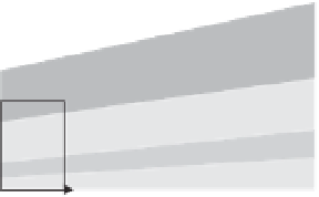
Outer region
y
Log-law layer
Buffer layer
Viscous sub-layer
6.2.6 Boundaryconditions
δ
Inner region
x
While the domain describes the physical extent of the flow
field, the values of the field variables (velocity, pressure,
turbulence quantities, etc.) need to be specified at the
boundaries. The most common and easiest to implement
specify a fixed value of a variable at the boundary which
is known mathematically as a Dirichlet condition (Smith,
1978). In CFD, the most obvious example is a fixed veloc-
ity at an inlet. At a flow outlet it is more difficult to specify
conditions. It can be said that, for a steady-state problem,
the outflow must equal the inflow or that the flow profile
must be uniform in the along stream direction. The latter
would require that the outlet is sufficiently downstream
of the area of interest and, if this is so, a condition on the
derivative of the along stream velocity may be imposed.
This problem must be approached carefully, in order
to prevent poor convergence or unphysical solutions.
Another condition, common in CFD, is a symmetry con-
dition, which may be used to allow for solution of only
half of a symmetric domain by imposing zero deriva-
tives on all variables except velocity into the symmetry
plane which has a value of zero. Before making use of a
symmetry plane it must be certain that the flow solution
will be symmetric - a symmetric domain and boundary
conditions do not guarantee a stable, symmetric solution.
Other boundary conditions occur, such as periodic and
shear free, and readers are referred to CFD texts (Versteeg
and Malalasekera, 2007) for details of them.
In environmental flows, care must be taken to ensure
that the turbulence quantities are correctly specified at
inlets and that the inlet profiles are consistent with the def-
inition of roughness along the boundaries of the domain.
Figure 6.3
Schematic of the various layers in the boundary
layer close to a wall.
boundary layer and a model of flow in that region based
on experiment is used. This method sets values for veloc-
ity, pressure and turbulent quantities and replaces the
solution of the Navier-Stokes equations at that point.
It is assumed that at the point next to the wall,
y
p
,
the production and dissipation of turbulence are equal.
Using this assumption gives the following equations,
which are characterized by a logarithmic profile for the
nondimensionalized velocity,
u
+
:
U
p
u
τ
1
κ
u
+
=
ln(
Ey
p
),
=
(6.9)
where
E
is a constant determined from experiment,
,is
von Karman's constant,
U
p
is the tangential component
of the velocity at a distance
y
p
from the wall, and
y
p
is the
nondimensionalized distance from the wall:
κ
τ
w
ρ
y
p
υ
y
p
=
,
(6.10)
τ
w
is the wall shear stress and
ν
where
is the kinematic
viscosity. Most codes apply this technique automatically,
but you need to watch out for what is actually being
done. If you are using wall functions, it is possible to
create a mesh that is too fine, which would mean that
your first point is in the viscous sub-layer which would
mean that you were using the wrong equation. However,
commercial codes now have wall functions that blend the
equations between the various layers of Figure 6.3.
The Law of the Wall can be amended to take account
of surface roughness, which is obviously important
in many environmental flows. Again, guidance can be
found elsewhere on appropriate values (Versteeg and
Malalasekera, 2007).
6.2.6.1 Wall functions
At a wall, the flow will be stationary and therefore there
will always be a narrow boundary layer of laminar flow,
which is known as the viscous sublayer, as shown in
Figure 6.3. Above it, there is a buffer layer and turbulent
boundary layer (labelled as the log-law layer in the figure
for reason that will become apparent). To resolve both
the viscous sublayer and the turbulent boundary layer
would require very fine meshes.
Wall functions are the answer to this problem and rely
on the use of the Law of the Wall. In this approach, the
mesh point next to the wall is placed in the turbulent
6.2.7 Post-processing
Visualization is one of the great strengths of CFD,
but can also be one of its downfalls in inexperienced
hands. The knowledge of field variables in each cell in


Search WWH ::

Custom Search