Information Technology Reference
In-Depth Information
10
6
1
2
3
4
5
6
7
8
9
10
10
5
10
4
10
3
10
2
10
1
10
0
10
0
10
1
10
2
Size
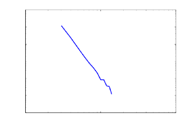
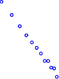
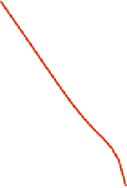
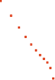
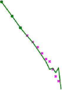
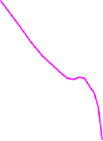
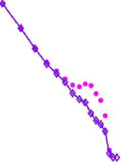
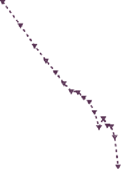
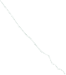
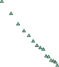
Fig. 12.3.
Distribution of the maximal cliques
Table 12.5.
Comparison between different schedules
G
Naive Schedule on
P
30
Random schedule on
P
30
Improvement
1
16
4
75%
2
4
1
76%
3
10
6
40%
4
21
18
14.28%
5
59
18
69.49%
6
171
169
1.16%
7
65
43
33.85%
8
132
64
51.52%
9
51
24
52.94%
10
198
98
50.50%
of all the maximal cliques obtained from the 10 graphs in Table 12.4 whose size
varies from 3 to 21 respectively.
In Fig.12.4,
X
axis is the size of the maximal clique.
Y
axis is the corre-
sponding number. We see that the call graph also has a power-law distribution
of its maximal cliques. We have compared our schedule mechanism with the
naive sequential schedule in Table 12.5. These experimental results are based on
the cellphone call networks in Table 12.4 as well. Here we see that our schedule
improves the whole eciency by a factor of 46.37% on average.