Environmental Engineering Reference
In-Depth Information
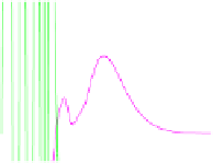
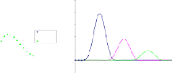
very strong oscillations are observed in the numerical response shown in Figure
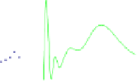
13.6c. This solution is unacceptable, owing to the magnitude of oscillations. Figure
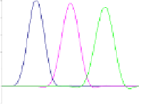
13.6d concerns the same purely convective problem (
Pe
= ∞) as indicated in Figure
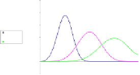
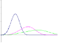
13.6a, but now pollutant degradation is taken into account. As in Figure 13.6b, the
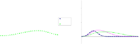
two last figures, 13.6e and 13.6f, concern a dispersive problem, but with an effect
related to immobile water. The mobile water concentration therefore diminishes
more rapidly than in Figure 13.6b, showing that part of the pollutant concentration
is stored in the immobile water (Figure 13.6f).
1.0
1.0
0.8
0.8
0.6
0.6
t= 2.5 sec
t=10.0 sec
t=17.5 sec
t= 2.5 sec
t=10.0 sec
t=17.5 sec
0.4
0.4
0.2
0.2
0.0
0.0
-0.2
-0.2
a: mobile water concentration,
b: mobile water concentration,
Cr=0.5, Pe=∞, no degradation effect, no
immobile water effect
Cr=0.5, Pe=2, no degradation effect, no
immobile water effect
1.0
1.0
0.8
0.8
0.6
0.6
t= 2.5 sec
t=10.0 sec
t=17.5 sec
t= 2.5 sec
t=10.0 sec
t=17.5 sec
0.4
0.4
0.2
0.2
0.0
0.0
-0.2
-0.2
c: mobile water concentration,
d: mobile water concentration,
Cr=2.5, Pe=∞, no degradation effect, no
immobile water effect
Cr=0.5, Pe=∞, with degradation effect, no
immobile water effect
1.0
1
0.8
0.8
0.6
0.6
t= 2.5 sec
t=10.0 sec
t=17.5 sec
t= 2.5 sec
t=10.0sec
t=17.5 sec
0.4
0.4
0.2
0.2
0.0
0
-0.2
-0.2
e: mobile water concentration,
f: immobile water concentration,
Cr=0.5, Pe=2, no degradation effect, with
Figure 13.6.
Time evolution of a pollutant pulse in a one-dimensional velocity field
Cr=0.5, Pe=2, no degradation effect, with