Environmental Engineering Reference
In-Depth Information
9.3.4.
Infiltration theory
We will now see how the notions introduced up to now in this chapter can be
applied in order to understand, mathematically formalize and, eventually,
numerically simulate an infiltration phenomenon in stone.
For this purpose, we will consider the example of a measuring test developed to
determine the so-called
capillary absorption coefficient
of a stone sample: it is the
RILEM test II.6 [RIL 80] routinely used to characterize the water behavior of a
stone (see numerous examples in [BOU 79, DES 95, HAM 93, MER 91]). In this
test, imbibition occurs in a stone sample that was initially dry. The position
z(t
) of
the wetting front is permanently monitored, together with the overall increase in
mass ∆
m(t)
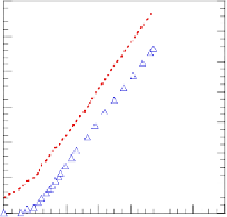
of the sample. Afterwards, to analyze the results of this test, these two
functions are plotted against the square root of time (see Figure 9.11). If the test was
run correctly, a straight part must be observed on both curves, as shown in this
figure. The slope of the straight line fitted on ∆
m
(√
t
) divided by the infiltrating
surface
s
of the sample defines the capillary absorption coefficient
A
[kg.m
-2
.s
-½
]
that was sought.
60
160
140
50
120
40
100
30
80
20
60
Wetting front
height
10
40
Mass intake
0
20
20
40
60
80
100
120
140
Square root of time (s
1/2
)
Figure 9.11.
Example of measurement of the capillary absorption coefficient A on a
“Tuffeau” sample. Here, a value for A = 0.6 kg.m
-2
.s
-0.5
has been fitted
To explain why these straight lines are always observed, the simple model of a
single cylindrical pore full of water (see Figure 9.3) is often invoked. Combining
Laplace's [9.7] and Poiseuille's laws [9.19], Washburn's equation is then obtained
[JEA 97]: