Blade Design, Manufacture, and Testing - Small Wind Turbines: Analysis, Design, and Application - page 131

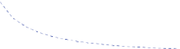
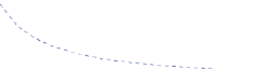
Fig. 7.4 a Chord
distributions for non-
dominated blades for the
values of a indicated for
Q r = 0.5 Nm. Solid line
shows Eq. 5.12 and the
dashed line shows ( 5.12 ).
Successive plots are
displaced upwards by 0.2.
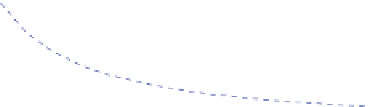
b Twist distributions for
non-dominated blades for the
values of a indicated for
Q r = 0.5 Nm. Solid line
shows Eq. 5.13 and the
dashed line shows ( 5.13 ).
Successive plots are dis-
placed upwards by 25

(a)

Q r = 0.5 Nm

0.6

a = 0.8

0.4

a = 0 . 9

0.2

a = 1.0

0

0.2 0.4 0.6 0.8 1

Radius, r/R

(b)

80

Q r = 0.5 Nm

a = 0.8

60

40

a = 0.9

20

a = 1.0

0

0.2 0.4 0.6 0.8 1

Radius, r/R

The inertia of the three blades for this design is 0.488 kgm 2 , which obviously
neglects the small contribution from the blade attachment. This is much greater
than the generator inertia given in Table 7.1 . This large difference has been
mentioned several times in previous chapters and is partly the reason why the
starting of a turbine with no resistive torque is independent of N, see Chap. 6 .
A designer particularly keen to improve low wind performance would probably
use the a = 0.8 blade, with 4% less power for a further 8% reduction in starting
time. By slightly increasing R, and redoing the optimisation, it would be possible
to further reduce the starting time at modest reduction in efficiency. Nevertheless,
the best trade-off between power extraction and starting is limited to a C 0.9
approximately, for both values of Q r .
An actual example of a dual-optimised blade is shown in the top part of
Fig. 7.6 . It is the 2.5 m long blade designed by the author for the two-bladed
Aerogenesis 5 kW wind turbine. The bottom part of the figure shows a 61.5 m LM
Glassfiber blade for large three-bladed machines. The smaller blade has signifi-
cantly greater chord over the whole blade—recall from Chap. 6 that optimum