Starting and Low Wind Speed Performance - Small Wind Turbines: Analysis, Design, and Application - page 109

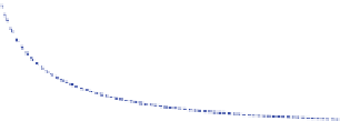
Fig. 6.8 Starting time and
the mean wind speed of 665
measured starting sequences,
and the predicted curves
using the three simulation
methods assuming steady
U [ 1 ]. The predictions (a),
(b), and (c) are by the
methods used in Fig. 6.4

180

160

measured data
prediction (a)
prediction (b)
prediction (c)

140

120

100

80

60

40

20

0

3 4 5 6 7 8 9 10 11 12

mean wind speed (m/s)

tan / U

Xr ¼ 1 kr ¼ 1

ð 6 : 14 Þ

k r

so that

a ¼ da

rU
r 2 X 2 þ U 2

dX
dt dt ¼

ð 6 : 15 Þ

With the data used to assess the importance of the rotor kinetic energy, and
c = 0.128 at the hub, r = 0.25 m, and c = 0.043 m at the tip, r = 0.97 m,
k & 8.5 9 10 -5 at the tip and 8.4 9 10 -5 at the hub. These values are too low to
cause the lift and drag to deviate from quasi-steady values [ 3 ].
Equations 4.6 and 4.7 with A = B = C = 1 provide the easiest treatment of
starting and are the only ones used here. Wright [ 1 ] found that these equations had
to be modified for the turbine in Fig. 6.1 with its relatively low aspect ratio of
about 9.0. Recent measurements of the starting of 2.5 m long blades with
AR = 14.3 were best reproduced with the high lift equations to be used here as
shown at the end of this chapter. Equation 6.3 becomes
dQ
dr ¼ NqU 2

1 = 2 cr sin h p cos h p k r sin h p

1 þ k r

ð 6 : 16 Þ

after some elementary manipulation to remove a and / in favour of h p .
When all lengths are normalised by the blade tip radius, R, and all velocities by
U,( 6.16 ) the equation for Q, the aerodynamic torque acting on the starting rotor, is

Q ¼ NqU 2 R 3 Z

1

1 = 2 cr sin h p cos h p k r sin h p dr

1 þ k r ð 6 : 17 Þ

r h

Equation 6.17 is probably too messy to integrate analytically even when cr is
constant. Nevertheless, it has several interesting consequences. First, the starting
time, say the time taken for the rotor to accelerate from rest to a specified tip speed
ratio, should be linear in the number of blades as long as solidity effects do not
alter the blade element lift and drag. Secondly, the starting time should scale
as U -2 , as is demonstrated in Fig. 6.8 . Thirdly, it is easy to show that Q has a local