Biomedical Engineering Reference
In-Depth Information
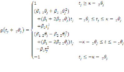
i in wh ich
β
1
= 1.0 020101308531,
β
2
=
−0.251006075157012,
κ
= 1.99607103795966.
Letting
t
j
=
x
m
w
j
' and substituting
t
=
t
j
+
2
θ
j
into
equation (9), we get the following
Data Set
The whole data set, denoted by
S
1
, contains 71
sets of measurements from 29 rivers in the United
States (Deng et al., 2001; Rowinski et al., 2005;
Seo & Cheong, 1998; Tayfur & Singh, 2005).
Apart from the longitudinal dispersion coef-
icient
K
, a reach mean parameter, there are five
independent variables. These are channel width
(
B
), flow depth (
H
), velocity (
U
), shear velocity
(
u
*) and river sinuosity (
α
= channel length/valley
length). Dependant variables are width-to-depth
ratio (
B
/
H
), relative shear velocity (
U
/
u
*) and
channel shape variable (
β
=
ln
(
B
/
H
)); a total of
eight variables are available.
The range for the dispersion coefficient (
K
)
varies from 1.9 to 892
m
2
/s
, and
K
is greater than
100
m
2
/s
in 21 cases, which represents about 30%
of the total measured coefficient values. The range
for the width-to-depth ratio (
B
/
H
) of the data sets
varies from 13.8 to 156.5 and (
B
/
H
) is greater than
50 in 26 cases. Other statistical information about
S
1
can also be found in Table 1.
S
1
is divided into two sub-sets,
S
1
t
and
S
1
v
for
training and validation/testing respectively.
S
1
t
contains 49 data sets out of 71, while
S
1
v
consists
of the remaining 22. When forming these two
sub-sets, the present work follows that of Tayfur
and Singh (2005), in order to compare results.
However, as mentioned in Tayfur and Singh
(2005): “In choosing the data sets for training
and testing, special attention was paid to ensure
that we have representative sets so as to avoid
bias in model prediction” (p. 993). Statistics for
S
1
t
and
S
1
v
are also listed in Table 1. As well as
the statistics in Table 1, it is worth mentioning
that the percentages of
K
> 100 m/s
2
and
B
/
H
>
50 are also comparable for both
S
1
t
and
S
1
v
. For
example, in
S
1
v
25% of
K
is greater than 100 m/s
2
(this ratio is 31% in
S
1
t
), also, in
S
1
v
40% of
B
/
H
is
greater than 50 (this ratio is 31% in
S
1
t
).
(10)
Thus for the
j
-th hidden neuron, the output
value is approximated with a polynomial form of
single variable
t
j
in each of four separate polyhe-
drons in the
x
m
space. For example, if
x
m
{
x
m
:
−
2
θ
j
≤
x
m
w
j
' ≤
κ
−
2
θ
j
}, then tanh (
x
m
w
j
' +
2
θ
j
) is
approximated with
β
12
θ
j
+
β
22
θ
j
2
+ (
β
1
+ 2
β
22
θ
j
)
t
j
+
β
2
t
j
2
. Because the activation function for the
output layer is a linear function, a comprehensible
regression rule associated with a trained ANN
with
i
hidden neurons is thus:
•
IF
x
m
{
x
m
: −
2
θ
j
≤
x
m
w
j
' ≤
κ
−
2
θ
j
for all
j
}
•
THEN
Thus, once the training is done the neural net-
work simulated output for
x
can be easily obtained.
In other words, regression rules associated with
the trained MLP can be derived.
CASE STUDy APPLICATION
In this case study, GNMM is applied to a very well
studied set of data. By comparing the results gener-
ated by GNMM to those in the literature, we aim
to demonstrate the effectiveness of GNMM.


Search WWH ::

Custom Search