Biomedical Engineering Reference
In-Depth Information
INTRODUCTION
However, owing to the requirement for de-
tailed transverse profiles of both velocity and
cross-sectional geometry, equation (1) is rather
difficult to use. Furthermore, equation (2), called
the method of moments (Wallis & Manson, 2004),
requires measurements of concentration distribu-
tions and can be subject to serious errors due to
the difficulty of evaluating the variances of the
distributions caused by elongated and/or poorly
defined tails. As a result, extensive studies have
been made based on experimental and field data
for predicting the dispersion coefficient (Deng,
Singh, & Bengtsson, 2001; Jobson, 1997; Seo &
Cheong, 1998; Wallis & Manson, 2004).
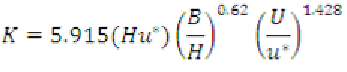
For example, employing 59 hydraulic and
geometric data sets measured in 26 rivers in the
United States, Seo and Cheong (1998) used di-
mensional analysis and applied the one-step Huber
method, a nonlinear multi-regression method, to
derive the following equation:
An important application of environmental hy-
draulics is the prediction of the fate and transport
of pollutants that are released into watercourses,
either as a result of accidents or as regulated dis-
charges. Such predictions are primarily dependent
on the water velocity, longitudinal mixing, and
chemical/physical reactions etc, of which longi-
tudinal dispersion coefficient is a key variable
for the description of the longitudinal spreading
in a river.
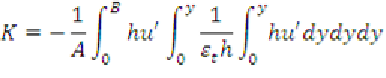
The concept of longitudinal dispersion coef-
ficient was first introduced in Taylor (1954). Based
on this work, the following integral expression
was developed (Fischer, List, Koh, Imberger, &
Brooks, 1979; Seo & Cheong, 1998) and gener-
ally accepted:
(1)
(3)
where
K
= longitudinal dispersion coefficient;
A
= cross-sectional area;
B
= channel width;
h
= local flow depth;
u'
= deviation of local depth
mean flow velocity from cross-sectional mean;
y
= coordinate in the lateral direction; and
ε
t
= local
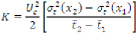
(depth averaged) transverse mixing coefficient. An
alternative approach utilises field tracer measure-
ments and applies the method of moments. It is
also well documented in the literature (Guymer,
1999; Rowinski, Piotrowski, & Napiorkowski,
2005; Rutherford, 1994) and defines
K
as
in which
u
* = shear velocity. This technique uses
the easily measureable hydraulic variables of
B
,
H
and
U,
together with a frequently used parameter,
extremely difficult to accurately quantify in field
applications,
u
*, to estimate the dimensionless
dispersion coefficient
K
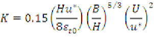
from equation (3). An-
other empirical equation developed by Deng et
al. (2001) is a more theoretically based approxi-
mation of equation (1), which not only includes
the conventional parameters of (
B
/
H
) and (
U
/
u
*)
but also the effects of the transverse mixing
ε
t0
,
as follows:
(2)
(4)
where
U
c
= mean velocity,
x
1
and
x
2
denotes up-
stream and downstream measurement sites, =
centroid travel time,
σ
t
2
(x)
= temporal variance,
where

Search WWH ::

Custom Search