Biology Reference
In-Depth Information
guideline. If more reality is added by way of a dynamic transmission term
that reflects a reduction in the rate of infection as a consequence of
treatment (the community wide effect of treatment), then Eq.
(9.4)
becomes more complex. One example based on no breakpoint and
a Poisson distribution of worm numbers gives the following expression:
f
f
1
1
R
f
0
1
t
f
z
L
0
1Þ
ln
þ
ln
(9.12)
1
ð
R
ð
R
0
1Þ
1
f
1
Here f is as defined in Eq.
(9.11)
, the time taken for the worm burden to
fall to a fraction f of the pre-treatment burden, e.g. 99%, L
1
is parasite life
expectancy in the human host (1/
m
1
) and 1
f
I
is treatment coverage.
46
Note that in the dynamic model transmission success in the community,
R
0
, now enters as an important variable in determining bounce-back time.
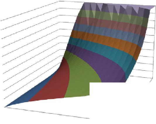
This is illustrated in
Figure 9.9
for various parasite life expectancies and
R
0
values. The importance of R
0
in determining the bounce-back time
highlights the importance of understanding the local context when
designing an intervention program. An obvious need is to extend these
analyses to try to get approximations for the bounce-back time t
f
, with
aggregated distributions of worms and mating probabilities inserted.
10
9-10
8-9
7-8
6-7
5-6
4-5
3-4
2-3
1-2
0-1
9
8
7
6
5
4
3
2
1
0
1.1
1.5
1.9
2.3
Ro
2.7
Coverage, 1-f
FIGURE 9.9
The average time taken for the average worm burden to bounce back to
80% of baseline, as in Eq.
(9.12)
for L
1
¼
1 year.
46
For low treatment coverage, 1
f
I
, and high
R
0
, bounce-back is very rapid (left), but for better treatment coverage, or lower R
0
it is
slower.


