Biology Reference
In-Depth Information
worm load in this model. Recent analyses have suggested that the weight
of female worms also affects this relationship, but this has yet to be
captured in transmission models.
29
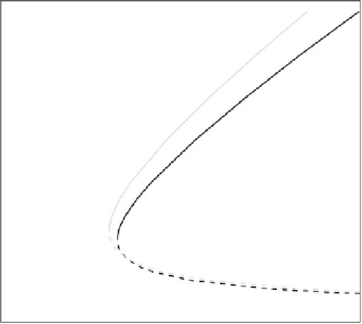
The properties of the simple model are revealed using conventional
methods to examine stability and dynamical behavior. The system has
two stable equilibria. Either there are no parasites, an equilibrium mean
worm burden of 0, or the system is at the equilibrium determined by R
0
and the other parasite characteristics, M* (solid lines on
Figure 9.5
). In
addition there is an unsteady state (dashed lines on
Figure 9.5
). If the
system starts above this line, parasite loads will increase to the usual
equilibrium. If, however, the system is perturbed to a state where the
mean worm burden is below this line (e.g. by an extremely successful
treatment program) then the population will crash to zero
e
i.e. the
k=0.9
k=0.7
k=0.4
1.2
1.4
1.6
1.8
2.0
R
0
FIGURE 9.5
Equilibrium worm burden as a function
R
0
for simple model (Eq.
9.6
)
and different values of worm distribution shape parameter,
k
. Solid lines represent stable
worm burdens and broken lines unstable burdens. In a population with a given R
0
, if worm
burdens can be brought below the dotted line by interventions, then the breakpoint has
been crossed and the cycle of transmission halted, leading to extinction. However, if worm
burdens are not reduced to this level, the system will return to the stable equilibrium,
increasing to baseline levels. The higher the level of aggregation (smaller k) the lower the
breakpoint. These plots are generated for the model expressed in Eq.
(9.6)
with the
parameters 1/(
m þ m
1
), the life expectancy of the worm in the human host, of 1 year and
fecundity parameter,
g ¼
0.05.