Image Processing Reference
In-Depth Information
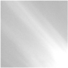
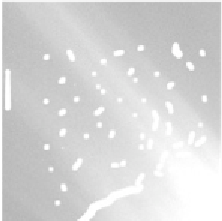
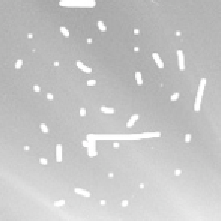
Figure 9.6
Examples of two pairs of training images. The images on the left are clean data.
The images on the right are the same pictures with representative noise added. In total, ten of
these sets were used in the training process.
Figure 9.6 shows examples of training images used. The images on the left are the
original clean ideal images and the ones on the right are the corresponding noisy
images created by adding patches of noise manually.
9.3.2 Training
Having created the training set, the next step was to carry out the training process.
This was performed using a combination of Matlab and C++ functions. Matlab
functions were used to make the overall procedure more scriptable. C++ functions
were used for the more computationally intensive parts of the GA to improve the
performance of the system.
The genetic algorithms operate by modeling the evolutionary processes found
in nature. The filter parameters (
, and
r
) were encoded into a binary string. A
fixed number of bits were used to represent the values within the hard center, the
soft surround, and the repetition parameter. Collectively these are known as a chro-
mosome.
At the beginning of the training procedure, a population consisting of thirty of
these chromosomes was created using a pseudo-random number generator. Each
chromosome was translated to a different filter that was applied to the noisy image
and its performance was evaluated. The genetic algorithm then proceeded to model
α
,
β