Information Technology Reference
In-Depth Information
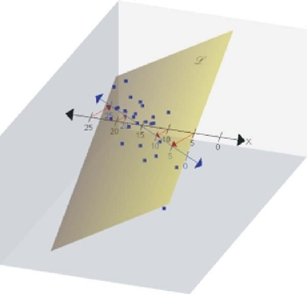
Figure 3.8
Constructing interpolation axis
X
in the biplot space.
As the plane
N
is shifted along the Cartesian axis
X
, a series of parallel intersection
spaces is obtained, as shown in Figure 3.15. Any line passing through the origin will pass
through these intersection spaces and can be used as a prediction axis fitted with markers
according to the value associated with the particular intersection space. To facilitate
orthogonal projection onto the axis, similar to an ordinary scatterplot, the line orthogonal
to these intersection spaces is chosen. For the data in Table 3.3 the prediction biplot axis
is shown in Figure 3.16.
The call
PCAbipl(X = as.matrix(Table.3.3.data[,-1]), ax.type =
"predictive", pch.samples = 15, pos = "Hor", offset =
c(0.1, 0.3, 0.3, 0.3), reflect = "y", colours = "green",
offset.m = rep(-0.25, 3), predictions.sample = c(9,24),
ort.lty = 2)
results in the predictive PCA biplot in Figure 3.17 of the data in Table 3.3. Note that for
PCAbipl
the default type of axis is
ax.type = "predictive"
.
Now that the biplot basics have been illustrated by the specific construction of a
PCA biplot, the next step is to evaluate how well the PCA biplot represents the original
centred data matrix
X
.