Information Technology Reference
In-Depth Information
r
0
−
2
g
5.5
RGF
0
q
0.1
SLF
u
5
v
3.5
3.5
h
2
m
p
j
c
4.5
3
2
2.5
i
4
f
1.5
1
n
0.2
b
0.5
4
a
0
6
d
k
3.5
w
s
e
8
SPR
0.3
3
t
PLF
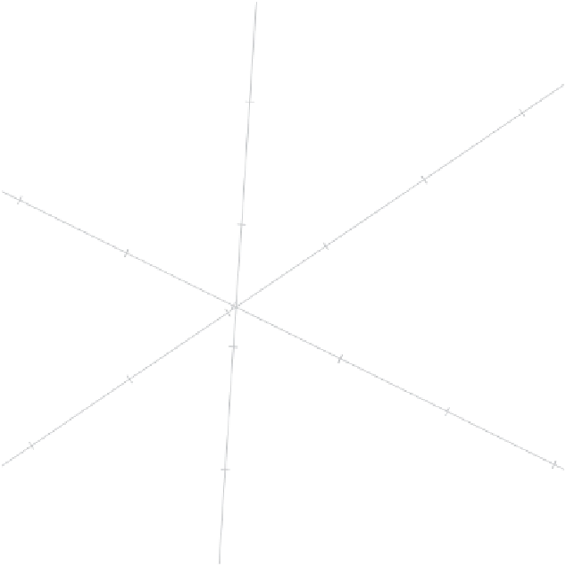
Figure 2.17
The biplot of Figure 2.16 but with the biplot axes calibrated in the original
units of measurement.
Opposite to prediction, we have the process of
interpolation
where axes are utilized to
place a (new) sample point by vector addition in the display. With an ordinary Cartesian
scatterplot, we use the single set of calibrated orthogonal axes for both interpolation and
prediction; however, this is invalid with the
p
nonorthogonal biplot axes.
In Figure 2.21, the process of prediction is illustrated in part (a). When interpolating
the values obtained in (a) by completing the parallelogram, a different sample represen-
tation is obtained in (b). In parts (c) and (d), this process is repeated for the sample
representation in (b). It is clear that a single set of nonorthogonal axes for both interpola-
tion and prediction results in inconsistent representation of the same sample point. For this
reason, generally biplots have to be equipped with different axes for prediction and for
interpolation. It is important to remember to use the correct set of axes when performing
predictions or interpolations. All the biplots considered thus far in this chapter have been
equipped with prediction axes, resulting in valid predictions from the given biplot axes.
In order to interpolate a (new) sample whose values are given in a
p
-component row
vector
x
into one of the biplots considered in this chapter, its coordinates relative to
the scaffolding of the biplot are given by
x
V
r
=
x
(
VJ
)
r
. This is trivial to compute, so
x
may be easily interpolated and shown on any computer screen or printout. However,
when away from the computer, some visual method of interpolation may be useful. It is