Information Technology Reference
In-Depth Information
2
−
r
−
2.5
g
−
2
RGF
−
1
−
1.5
q
1
SLF
−
1
u
v
h
j
c
−
0.5
1
m
p
i
f
0
n
−
1
b
0.5
a
−
2
−
1
1
d
1
k
w
1.5
s
e
2
−
SPR
2
t
2
PLF
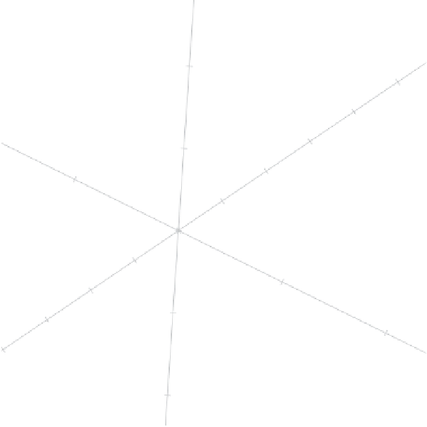
Figure 2.16
Two-dimensional biplot of the normalized aircraft data as given in Table 2.2
with scales in the normalized units.
= c(8,9,13)
to predict the
SPR
,
RGF
,
PLF
and
SLF
for aircraft
h
,
i
and
n
from the
biplot axes in Figure 2.17. This is shown in Figure 2.20.
When argument
predictions.sample
is not set to
NULL
the biplot function not
only shows explicitly the orthogonal projections onto the biplot axes as illustrated in
Figure 2.20 but also returns the actual predictions made. The output resulting from
setting
predictions.sample = c(8,9,13)
is shown in Table 2.3 together with the
actual values. As an exercise, the reader may check that these predictions remain exactly
the same regardless of applying orthogonal parallel translation, reflection or rotation.
Ta b l e 2 . 3
Predicted
SPR
,
RGF
,
PLF
and
SLF
values for aircraft
h
,
i
and
n
together
with the corresponding actual values in Table 1.1.
Predictions
Actual values
s8
s9
s13
h
i
n
SPR
2.5266
2.6768
4.9705
2.426
2.607
5.855
RGF
4.4299
4.1956
4.6644
4.650
3.840
4.530
PLF
0.1108
0.1597
0.1947
0.117
0.155
0.172
SLF
2.0847
1.7540
2.6307
1.800
2.300
2.500