Information Technology Reference
In-Depth Information
We illustrate the principles for linear axes, but they may be readily extended to other
cases. Figure 2.5 is plotted, as is usual, in such a way that the centroid of the points is at
the origin. This is a natural choice of origin because it is known that the best fit of (2.1)
passes through the centroid of all the points. However, it does tend to force the axes, with
their scale markers, to intermingle with the points, which does not help legibility. As all
we wish to do is to project orthogonally onto each axis, any axis may be moved parallel
to itself - provided we ensure that the markers are moved consistently. By 'consistent'
we mean that the line joining the same marker on two parallel axes is orthogonal to them
both, as is shown in Figure 2.11. We call this process
orthogonal parallel translation
.
The axis may be made to pass through any chosen point (a, b) relative to the plotting
axes and the same point (a, b) may be chosen for all axes, thus ensuring concurrency. By
choosing judiciously, we may take advantage of this simple fact to separate the axes from
the points, as is shown in Figure 2.12, resulting in an improved Figure 2.5. Complete
separation is always possible but not always desirable when it induces a remote origin
just to accommodate separation of a few points. Furthermore, the plotting area needs to
be enlarged to facilitate reading off the values of samples
w
and
s
.
SLF
RGF
6
6
5
4
5
r
c
0.1
3
j
q
p
k
m
u
g
v
2
i
h
t
n
d
4
f
e
s
w
1
0.2
b
a
0
3
−
1
0.3
2
−
2
4
SPR
PLF
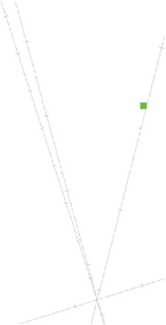
Figure 2.12
Biplot of the aircraft data with orthogonal parallel translation of the axes
to separate the axes from the samples.