Information Technology Reference
In-Depth Information
−
0.04
−
0.02
0
11
0.02
1sd
0.04
0.06
0.08
0.1
0.12
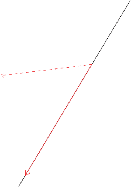
Figure 2.8
Calibrating a biplot axis. Similar to Figure 2.7 but with
lambda = 3
and
shift = 0.1.
The origin is indicated by the green circle. The calibration marker '1sd'
approximates a distance of one standard deviation from the origin. The actual standard
deviation is 0.0305.
is approximated by the intersection of the blue dotted line and the red arrow, but the
calibrations are transformed into the original scale using the calibration procedure. The
point '1sd' approximates the transformed mean of zero plus the transformed standard
deviation of unity, but the calibration is in terms of the original mean of 0.0347 plus
the original standard deviation of 0.0305. Since
V
2
V
2
approximates
VV
=
I
,whichis
the covariance matrix of the scaled data, the tip of the red arrow coincides in Figure 2.9
with the position of the point '1sd', but this is not so in Figure 2.10.
The calibration of the biplot axes in Figure 2.9 may seem a trivial operation, but let
us take a closer look at the principles involved. Useful scale values should be in terms
of the original data but the biplot scaffolding is in terms of the normalized data matrix.
'Nice' scale values of the first column of our original data matrix are thus needed and not
those of the first column of
X
Norm
. The values in the first column of
X
Norm
range over
the interval [
3.0304;3.2016]. The R function
pretty
allows us to obtain the required
nice values 0.00, 0.02, 0.04, 0.06, 0.08 easily using the instruction
−
>
markers.x <- pretty(range(X[,1]), n = 5)