Information Technology Reference
In-Depth Information
SLF
RGF
6
0
6
5
4
0.1
r
5
q
c
3
p
j
2
k
m
u
g
v
i
h
t
4
2
n
d
0.2
6
f
4
e
s
w
1
8
SPR
b
a
0
0.3
3
−
1
PLF
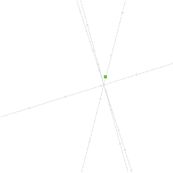
Figure 2.5
A two-dimensional biplot approximation of the aircraft data of Table 1.1
according to the Gower and Hand (1996) representation. Note the aspect ratio of unity.
Care has been taken with the construction of Figure 2.5 that the aspect ratio is equal
to unity. This is not shown explicitly, but the square form of this figure (and others) is
intended as an indication.
The main difference between the biplot in Figure 2.5 and an ordinary scatterplot is that
there are more axes than dimensions and that the axes are not orthogonal. Indeed, it would
not be possible to show four sets of mutually orthogonal axes in two dimensions. There
is a corresponding exact figure in four dimensions and the biplot is an approximation to
it. This biplot is read in the usual way by projecting from a sample point onto an axis
and reading off the nearest marker, using a little visual interpolation if desired. If the
approximation is good, the predictions too will be good.
Having shown a biplot with calibrated axes representing the original variables we
now give details on how to calculate these calibrations: whenever a diagram depends on
an inner product interpretation, the process of calibrating axes may be generalized as we
now show.
Calibrated axes are used throughout this topic for a variety of biplots associated
with numerical variables. We point out that a simple methodology is common to all