Information Technology Reference
In-Depth Information
RAC
Gaut
CrJk
Gaut
KZN
DrgR
CmRb
WCpe
AtMr
InAs
PubV
CmAs
0
WCpe
Arsn
Mrd
BRs
BNRs
Mpml
Rape
NWst
FrSt
E
Cpe
Limp
Mpml
NCpe
AGBH
2e 04
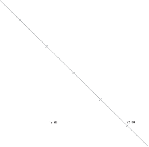
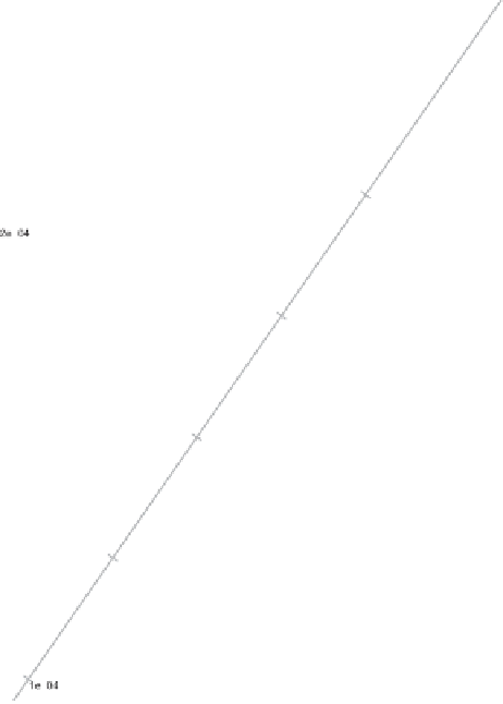
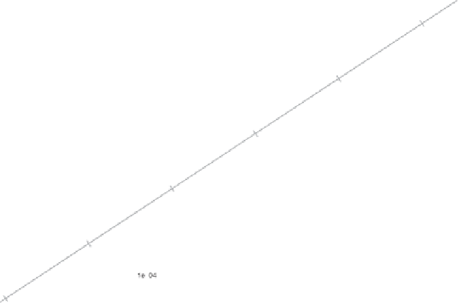
Figure 7.16
Similar to Figure 7.15 but plotting the provinces as calibrated axes with
the different crimes as points. Two-dimensional CA biplot of the 2007/08 crime data
set. Chi-squared distance approximation plotting
U
and
C
−
1
/
2
V
(column chi-squared
distance) with the argument
lambda = TRUE
. (Lambda evaluates to 0.0275).
The previous example raises the question of how to include the time aspect in a CA
biplot. Indeed, the full crime data set can be considered to be a three-way contingency
table. An obvious way is to concatenate the seven two-way contingency tables row-wise.
As an example of this we show in Figure 7.26 the Pearson residuals case A CA biplot
for the concatenated 2001/02 and 2007/08 crime data. This biplot shows some evidence
of a reduction in several of the crimes for most of the provinces: the main exceptions are
KZN
and
WCpe
, where the position of
KZN
indicates a large increase in murder and
that of
WCpe
a large increase in drug related issues. In order to understand this biplot,
as already stated, we have to take into account the calculated measures of fit: the overall
quality of the display is a satisfactory 84.65% (see Table 7.30); the column predictivities
and row predictivities are given in Tables 7.31 and 7.32.


