Information Technology Reference
In-Depth Information
CrJk
CrJk
R
A
C
Gaut
AtMr
e
CmRb
KZN
AtMr
InAs
DrgR
CmRb
InAs
DrgR
0
CmAs
WCpe
0
0
0
CmAs
Mrd
BRs
BNRs
Arsn
Mpml
Rape
AGBH
PubV
NWst
FrSt
NCpe
Limp
Arsn
ECpe
Figure 7.15
Two-dimensional CA biplot of the 2007/08 crime data set. Chi-squared
distance approximation plotting
U
and
C
−
1
/
2
V
(column chi-squared distance) with the
argument
lambda = TRUE
. (Lambda evaluates to 0.0264).
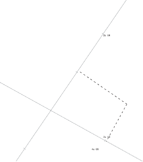
Before we can draw final conclusions on our comparison of the interpolated values
for the two provinces shown in Figures 7.22 and 7.23, we would like to know how well
the interpolated points are represented in the respective graphs. Although the interpolated
points do not contribute to the position of the axes, we can still answer this question by
considering how well the axes predict the actual values of the interpolated points. There-
fore, we first obtain the predictions for the interpolated values just as we have done in the
case of the original points. Setting the argument
predictions.X.new = TRUE
allows
us to find these predictions, as is illustrated in Figure 7.24 for the Western Cape province.
The actual values of the weighted Pearson residual matrix (see (7.2))
R
−
1
/
2
new
(
X
new
−
E
new
)
C
−
1
/
2
(7.54)


