Information Technology Reference
In-Depth Information
4e 05
RAC
AtMr
CrJk
CmRb
Gaut
InAs
KZN
DrgR
CmRb
AtMr
DrgR
InAs
CmAs
0
0
WCpe
0
PubV
CmAs
Arsn
BNR
BRs
Rape
Mrd
Mpml
NWst
FrSt
ECpe
Limp
NCpe
A
GBH
Figure 7.14
Two-dimensional CA biplot of the 2007/08 crime data set. Chi-squared
distance approximation plotting
R
−
1
/
2
U
and
V
(row chi-squared distance) with the
argument
lambda = TRUE
. (Lambda evaluates to 36.33).
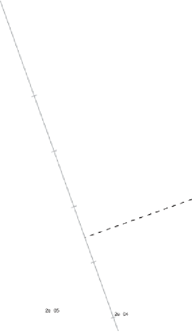
We now give some examples of interpolating new points in CA biplots. We
first form a set of points to interpolate by taking the crime data for the Wes-
tern Cape province for each of the periods 2001/02, 2002/03,
...
, 2007/08 and
arrange them as the rows of an R data matrix called
SACrimeWcpe.data
.Acall
to
cabipl
with arguments
X.new = SACrimeWcpe.data
and
X.new.labels
= c("02","03","04","05","06","07","08")
leads
to
the
biplot
given
in
Figure 7.22.
Notice that in Figure 7.22 the point representing the row for the 2007/08 data in
X.new
interpolates into its correct place. Of importance are the interpolated positions of
the other points: there is a clear progression of the interpolated points away from the
2007/08 point with the earlier data. Interpolating values for Gauteng province does not
show this tendency: see Figure 7.23.


