Information Technology Reference
In-Depth Information
CrJk
0
0.8
0.95
2
0.5
0.8
AtMr
RAC
0.5
0.5
CmRb
2
0.5
1.5
1.2
Gaut
1.2
1.5
InAs
AtMr
KZN
DrgR
DrgR
CmRb
InAs
3
1.5
WCpe
CmAs
BRs
BNRs
1
1
2
0.9
CmAs
Mrd
0
0.5
0.8
0.5
Arsn
Rape
FrSt
PubV
Mpml
0.8
NWst
1.5
0.5
ECpe
0
AGBH
0.6
Limp
1.5
1.5
0.6
NCpe
1.2
2
0
1.5
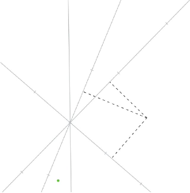
Figure 7.12
Two-dimensional CA biplot of the 2007/08 crime data set. The contingency
ratio is approximated by plotting
R
−
1
/
2
U
and
C
−
1
/
2
V
with correctly adjusted scales
and with the argument
lambda = TRUE
.
As an illustration, the row profiles of the 2007/08 crime data contingency table
are shown, in deviation form, in Table 7.21. Instead of approximating the row pro-
files directly, we can construct a biplot from
R
−
1
/
2
U
for the rows and
C
1
/
2
V
for the
2
for the
columns. Then, using the calibration tool, we can calibrate the axes in terms of the actual
row profiles. These different biplots are shown in Figures 7.18 - 7.20.
Figure 7.16 showed that in order to plot the rows of a contingency table as biplot
axes with the columns as points, all that is necessary is to transpose the data matrix as
input to the argument
X
of the function
cabipl
. As a further example of this we provide
Figure 7.21 as a CA biplot of the 2007/08 crime data set approximating the column
profiles (
X
-
E
)
C
−
1
. The biplot in Figure 7.21 can be considered as an approximation of
the profiles of the types of crime with the provinces as calibrated axes.
1
/
2
1
/
columns as described above, or from
R
−
1
/
2
U
for the rows and
C
1
/
2
V


