Information Technology Reference
In-Depth Information
0.6
CrJk
RAC
0.8
0.5
AtMr
2
0.5
CmRb
InAs
1.5
AtMr
0
0
2
DrgR
1.4
0.5
CmRb
0.5
2
0.5
InAs
1.5
1.2
0.5
DrgR
1.5
WCpe
Gaut
1
1
1
1
1
1
CmAs
KZN
1
2
1
0.8
1
1
1.5
3
0.8
CmAs
1
0.5
2
1
1
1
1.5
0
0.6
0.5
0.5
1.2
0
Mpml
BRs
NWst
ECpe
Limp
Mrd
FrSt
2
1.5
0
1.5
0.5
1.5
NCpe
BNRs
2.5
2
2
2
Arsn
PubV
1.5
Rape
1.5
AGBH
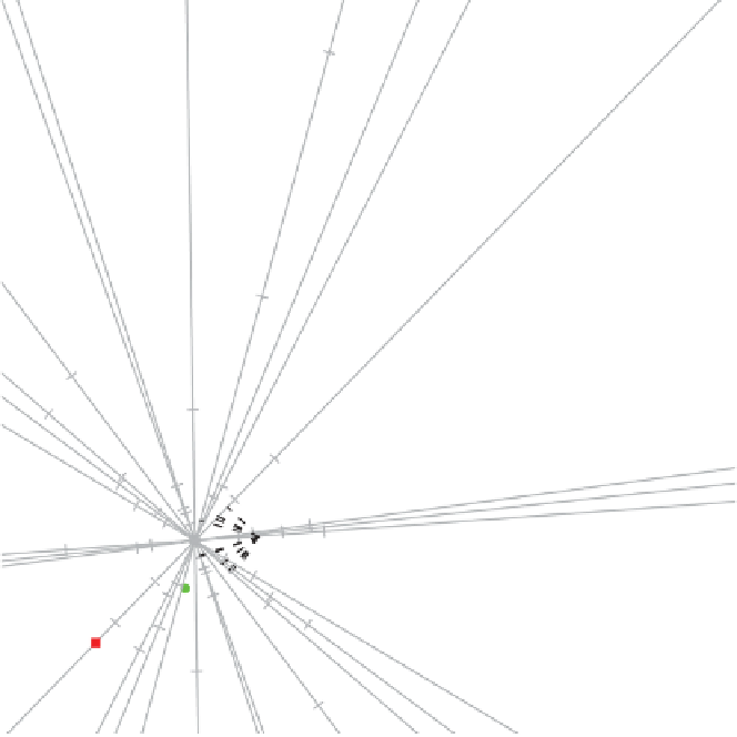
Figure 7.11
Two-dimensional CA biplot of the 2007/08 crime data set. The contingency
ratio is approximated by plotting
R
−
1
/
2
U
and
C
−
1
/
2
V
with correctly adjusted scales
and with the argument
lambda = FALSE
(the default).
The distances in Table 7.19 were calculated as follows. The biplot in Figure 7.15
provides the approximation to the matrix
R
−
1
/
2
(
X
-
E
)
C
−
1
. This approximation was used
for calculating the between-column chi-squared distances precisely in the same way as the
actual distances were calculated from
R
−
1
/
2
(
X
-
E
)
C
−
1
using the function
Chisq.dist.
In Figure 7.16 we have switched the role of the columns and the rows by providing
as input to
cabipl
the transposed matrix
X
, while the correlation approach discussed in
Section 7.2.5 is illustrated in Figure 7.17.
In Table 7.20 we show the first 10 rows of the matrix
G
: 1 104 159
×
23 of the
2007/08 crime data set. This matrix was constructed from the contingency table given in
Table 7.5 by using our function
indicatormat
for converting a contingency table into
indicator matrix form. The first nine columns of Table 7.20 are the indicator matrix for
the row categories and the last 14 columns that for the column categories.