Information Technology Reference
In-Depth Information
-2000
-1000
20000
4000
-2000
-500
-3000
-20000
Gaut
AtMr
1000
-2000
RAC
10000
2000
-500
-1000
CmRb
-10000
-50
-1000
2000
KZN
CrJk
InAs
DrgR
CmRb
500
DrgR
CmAs
WCpe
0
20000
0
0
-2000
AtMr
BRs
CmAs
PubV
Rape
InAs
Mr
d
Arsn
2000
-20000
-500
BNRs
NCpe
Mpml
NWst
FrS
Limp
-2000
50
1000
ECpe
-4000
10000
1000
-2000
-10000
100
500
-1000
2000
AGBH
Arsn
PubV
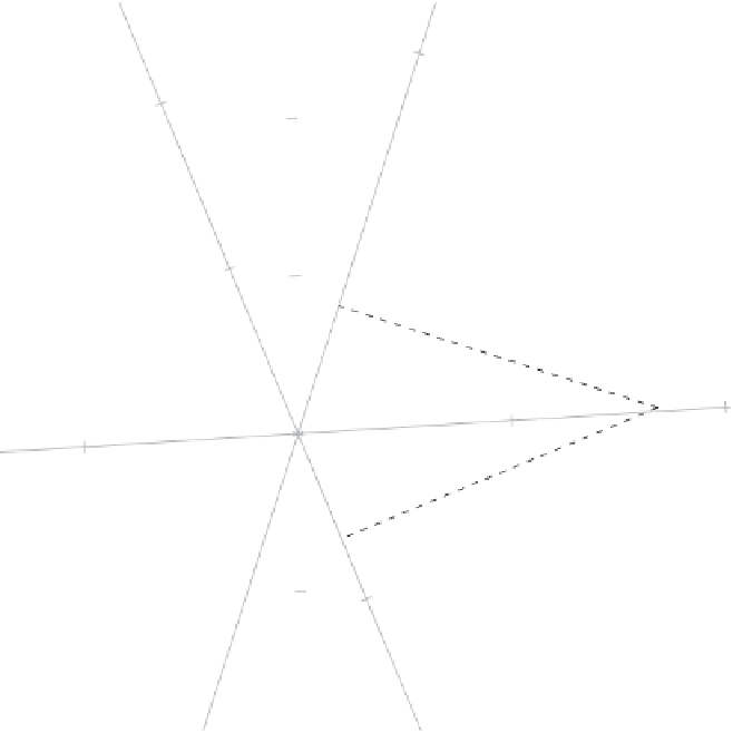
Figure 7.9
Two-dimensional CA biplot of the 2007/08 crime data set. Deviations from
independence are approximated by plotting
R
1
/
2
U
1
/
2
1
/
2
.
and
C
1
/
2
V
Since the deviance for a log-linear model is defined as
2
observed
×
log
observed
expected
,
(7.53)
it might be of interest to calibrate axes in terms of the logarithm of the contingency
ratio. Notice that this is an example of a linear axis with unequal spaced intervals.
Setting the argument
logCRat = TRUE
in the call to
cabipl
allows this functionality
by utilizing the calibration tool discussed in Section 2.3. Figure 7.13 provides an example
of approximating the contingency ratio in terms of a logarithmic scale. We set
ax=9
to suppress plotting of all the axes except the
DrgR
-axis in order to draw attention to
the calibrations on this axis.
In Table 7.16 we show
√
n
times the chi-squared distance matrix between the
rows of our 2007/08 crime data set. The corresponding biplots (setting the arguments