Information Technology Reference
In-Depth Information
100
-10
150
-20
-40
-100
RAC
100
-20
Gaut
50
AtMr
-20
CrJk
-50
-5
CmRb
50
-10
20
KZN
InAs
DrgR
CmRb
20
DrgR
AtMr
200
WCpe
-20
0
10
InAs
PubV
Mrd
100
CmAs
CmAs
Arsn
BRs
BNRs
0
-100
-10
Rape
-20
Mpml
NWst
NCpe
FrSt
5
-50
10
Limp
50
ECpe
5
-40
20
-50
Arsn
AGBH
10
-20
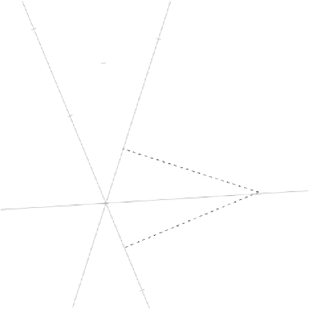
Figure 7.6
Two-dimensional CA biplot for the 2007/08 crime contingency table. Similar
to the biplot in Figure 7.5, but calibrations scaled by a factor of
n
1
/
2
using methods
described in Chapter 2. Thus, calibrations are in terms of Pearson residuals.
Ta b l e 7 . 1 1
Quality expressed as percentages for the 2007/08 crime
contingency table in weighted deviation form
R
−
1
/
2
(
X
−
E
)
C
−
1
/
2
.
Dim 1
Dim 2
Dim 3
Dim 4
Dim 5
Dim 6
Dim 7
Dim 8
Dim 9
56.67
87.84
94.24
96.49
98.49
99.44
99.88
100.00
100.00
It turns out from the output of
cabipl
that in this case
λ
=
1
.
9032, where
λ
is defined
by (7.52).
Figure 7.8 demonstrates the usefulness of the lambda tool and also that the biplot
resulting from plotting
U
and
V
conveys the same information as the one resulting from
plotting
R
1
/
2
U
2
. The above characteristics are also true for one- and
three-dimensional biplots. The reader can verify this by setting
dim.biplot = 1
(or
3
)
in the above calls to
cabipl
.
1
/
2
and
C
1
/
2
V
1
/