Information Technology Reference
In-Depth Information
t
0.3
s
u
v
w
0.2
q
n
d
j
0.1
c
e
k
p
0.0
m
h
5.5
r
i
8
5.0
f
b
6
4.5
g
a
4
4.0
2
3.5
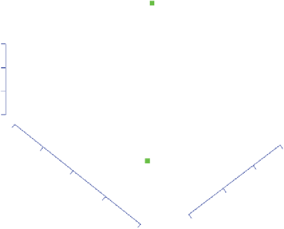
Figure 2.2
Three-dimensional scatterplot of variables
SPR
,
RGF
and
PLF
of the
aircraft data in Table 1.1.
Figure 2.3 shows the resulting plot where we have first subtracted the means of the
individual variables from each aircraft's measurements. The same plot appears in both
panels of Figure 2.3, the only difference being that the axes have been translated to pass
through the point (0, 0) in the bottom panel. The orthogonal axes give the directions
of what are known as the two principal axes. These mathematical constructs do not
necessarily have any substantive interpretation. Nevertheless, attempts at interpretation
in terms of
latent variables
are commonplace and sometimes successful. Any two oblique
axes may determine the two-dimensional space, so there is an extensive literature on the
search for interpretable oblique coordinate axes. Rather than dealing with latent variables,
biplots offer the complementary approach of representing the original variables. Clearly,
it is not possible to show four sets of orthogonal axes in two dimensions, so we are forced
to use oblique representations. The axes representing the latent variables will generally
not be shown; they form only what may be regarded as one-, two- or three-dimensional
scaffolding axes
on which the biplot is built.
How is Figure 2.3 constructed? The usual way of proceeding (Gabriel, 1971) is based
on the SVD,
X
:
n
×
p
=
U
∗
∗
(
V
∗
)
,
(2.1)
where, assuming that
n
≥
p
,
U
∗
is an
n
×
n
orthogonal matrix with columns known as
the left singular vectors of
X
, the matrix
V
∗
is a
p
×
p
orthogonal matrix with columns