Information Technology Reference
In-Depth Information
−
100
0
100
Tem
−
100
Cra.H(58)
−
50
0
−
80
Fow.H(12)
Ran
Edn.L(88)
Kin
50
Beg.L(80)
350
−
50
20
Cra.L(62)
−
100
−
50
50
Spo
Ear.H(15)
300
300
Edn.H(71)
T95
−
50
250
0
40
−
150
250
−
50
200
Hob
−
60
0
150
20
200
T64
0
0
−
200
−
200
T68
150
Dur
Hun
−
20
−
100
Cap
Fun
100
50
50
−
100
−
50
−
40
0
Ear.L(29)
Figure 6.13
Similar to Figure 6.12 but predicting the values (in terms of interactions
with main effects added) for all varieties at the same site (
Edn.H
). Accomplished by call-
ing
biadbipl
with arguments
X = t(wheat.data), predictions.allsamples.
onaxis = 12
.
biadditive family. Rather than operating on the interaction matrix
Z
, we now operate on
the original data
X
and use its SVD,
X
=
U
V
. When the simple additive model holds,
the matrix form of (6.1) is
X
=
µ
11
+ α
1
+
1
β
or, on rewriting,
X
=
(µ
1
+
α
)
1
+
1
β
,
which, being the sum of two products, shows that
X
is of rank 2. Thus, if we make a
biplot with coordinates (
µ
1
+ α
,
1
)and(
1
,
β
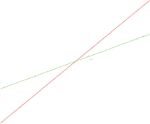
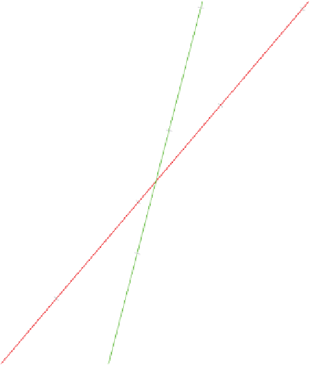
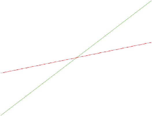
) we get two lines at right angles. The values
of
µ
,
α
,
β
are unknown but the SVD of
X
will exhibit the same orthogonal structure. The
converse is also true, that if the SVD exhibits this structure, then the underlying model
must be of simple additive form. This result may be used as a diagnostic for the additive
model (Bradu and Gabriel, 1978). In applications there will be variations in the data,
modelled by the usual error term, and the geometry will not be exact, but nevertheless
it remains useful.
In the general case where there is one biadditive term,
X
β
+
γδ
,
X
is of rank 3 and the two-dimensional biplot derived from the SVD exhibits no struc-
ture. Then we would infer that there was at least one biadditive term. There are two
11
+
α
1
+
=
µ
1


