Information Technology Reference
In-Depth Information
Fun(58)
Hun(62)
T68(15)
Dur(43)
T64(30)
−
100
Cap(72)
15
50
−
10
40
0
0
50
−
20
100
20
50
50
Hob(78)
−
−
30
Box.H
−
50
60
20
−
20
Spo(44)
25
0
T95(8)
0
Box.L
Tru.H
−
40
0
0
−
50
Tem(93)
0
−
50
Ear.L
Tru.L
−
50
−
100
50
Ear.H
Fow.H
Cra.L
Cra.H
Edn.H
Beg.L
−
15
0
−
100
Edn.L
10
Beg.H
Kin(75)
0
Fow.L
50
Ran(53)
Beg.H(48)
Fow.L(53)
Cra.H(58)
Beg.L(80)
Cra.L(62)
Ear.H(15)
40
40
150
Fow.H(12)
−
−
−
160
60
30
Edn.L(88)
−
50
300
−
1
00
Edn.H(71)
−
180
20
Tem
350
20
250
−
200
10
−
60
−
200
−
20
20
200
300
80
−
70
150
Ear.L(29)
0
80
−
−
50
250
Kin
0
Ran
0
200
0
Spo
150
20
Hob
T95
−
50
T64
Tru.H(71)
−
60
−
100
0
T68
Dur
Hun
Cap
Fun
50
−
40
0
Box.H(83)
Tru.L(21)
Box.L(62)
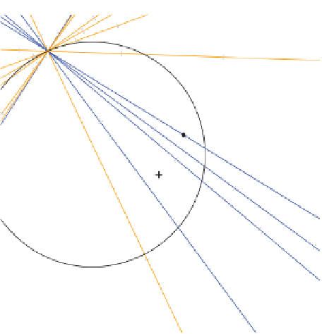
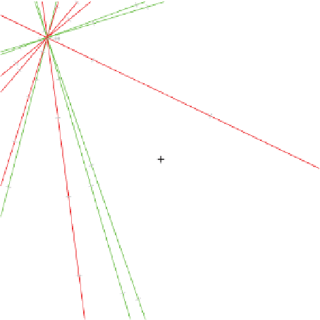
Figure 6.11
Similar to Figures 6.9 and 6.10, but with axes shifted as a result of setting
select.origin = TRUE
when calling
biadbipl
. Note that all predictions are exactly
as in Figures 6.9 and 6.10. This figure illustrates why it can be advantageous to have the
point of concurrency at or near the origin: all intersections of constructed circles with
axes would tend to appear on the biplot. Note also that the black solid circles representing
the main effects have moved with the axes and are no longer superimposed at the origin
that is marked with a black cross.