Information Technology Reference
In-Depth Information
−
50
Cra.H(58)
0
Tem
100
−
50
−
80
−
50
−
80
Ran
Kin
0
−
50
50
Spo
−
50
Beg.L(80)
T95
−
60
Cra.L(62)
Hob
0
T64
T68
Ear.H(15)
−
150
−
150
−
60
0
Dur
−
100
40
−
40
Fow.H(12)
20
Edn.L(88)
Hun
50
20
Cap
Edn.H(71)
−
200
−
200
300
Fun
250
−
100
50
200
0
−
100
−
20
250
150
50
0
Ear.L(29)
200
−
40
−
150
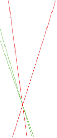
(b)
Figure 6.7
(
Continued
)
Knowledge of the size of the interaction is useful, but plant breeders will want to
know the absolute value of yield at each site. This is easily obtained by adding the site
main effect to the interaction, which can be readily achieved by adjusting the markers
on the site biplot axes. When this is done the actual main effect itself may be marked
by a special symbol. This is done in Figure 6.7, where we have also taken the oppor-
tunity to shift the axes to a position where the points representing the varieties are not
obscured by the axes and labels. Of course, the same could be done for the biplot showing
variety axes.
We have demonstrated that, just as we may evaluate axes predictivities for PCA,
so may we evaluate row and column predictivities for two-way tables - all we have to
do is to find the ratios of the sum of squares for the rows (or columns) of
X
to the
same sum of squares for the same rows (or columns) of
X
. In practice we would first
remove the overall mean from
X
. We have seen that it is also useful to remove row and
column main effects to provide for the residual matrix
Z
with its own row and column
predictivities. By projecting the variety points onto an environmental axis, we obtain
estimates of the interaction term. To get the total environmental effect, one may wish to
include the contribution of the environmental main effect in the biplot. To do so, one
merely has to shift the scale-markers by an amount equal to the magnitude of the main
effect. Thus, the total environmental contribution (main effects
+
interaction) may be
represented in a calibrated biplot. This has been done in Figure 6.7(b) where, at the same