Information Technology Reference
In-Depth Information
Fow.L(53)
Beg.H(48)
100
−
50
Cra.H(58)
Tem
−
50
−
20
50
50
40
−
Fow.L(53)
−
50
50
Fow.H(12)
Beg.H(48)
Edn.L(88)
20
Beg.L(80)
Ran
100
Kin
Cra.L(62)
Edn.L(88)
−
20
50
Cra.H(58)
50
50
Ear.H(15)
Edn.H(71)
Spo
Fow.H(12)
Beg.L(80)
20
50
T95
Edn.H(71)
Cra.L(62)
0
Ear.H(15)
Hob
0
−
50
−
50
T64
Tru.L(21)
Ear.L(29)
T68
−
20
−
100
−
50
20
−
50
Box.L(62)
Dur
−
20
Hun
Cap
50
Fun
Tru.H(71)
−
50
40
20
−
50
50
−
50
Ear.L(29)
Box.H(83)
50
100
Tru.H(71)
Box.H(83)
Tru.L(21)
Box.L(62)
T68(15)
Fun(58)
Dur(43)
Hun(62)
50
0
Box.H
0
Cap(72)
20
50
100
50
Box.L
Fun(58)
0
Tru.H
Hun(62)
0
Cap(72)
T64(30)
Dur(43)
0
T68(15)
Ear.L
50
Tru.L
20
0
T64(30)
0
50
Ear.H
Hob(78)
0
Hob(78)
Cra.L
Fow.H
B
eg.L
T95(8)
Edn.H
0
Spo(44)
0
Cra.H
Kin(75)
50
50
Edn.L
Ran(5
3
)
Beg.H
0
50
−
20
Fow.L
Spo(44)
0
50
100
T95(8)
Kin(75)
20
0
Tem(93)
Tem(93)
Ran(53)
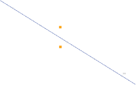
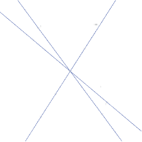
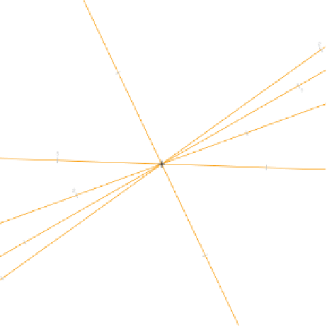
Figure 6.6
Extension of Figure 6.5. SVD of
Z
=
U
V
. In the top panel varieties are
plotted from first two dimensions of
U
2
using our R function
biadbipl
with arguments
X = wheat.data
,
biad.variant =
"InteractionMat"
,
SigmaHalf = TRUE
. Sites are also shown as calibrated axes.
Calibrations are in terms of interactions. Notice that each axis passes through zero and
one of the sites. Using a similar function call with
X = t(wheat.data)
results in the
biplot in the bottom panel. Note that in these biplots neither column points nor row points
are lumped together.
1
/
2
1
/
and sites from first two dimensions of
V