Information Technology Reference
In-Depth Information
Box.H
Cap
Fun
Dur
T68
Hun
T95
Hob
T64
Tru.H
Kin
Spo
Box.L
Ran
Tem
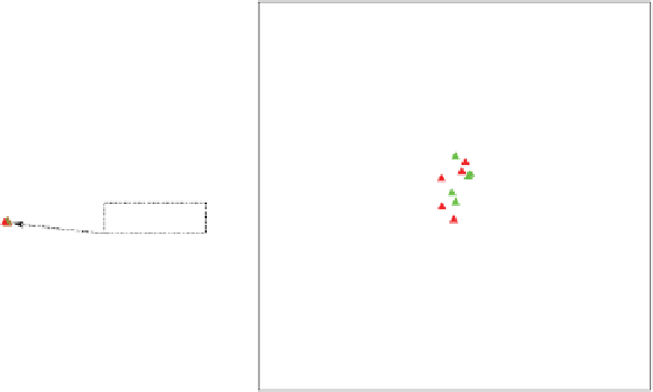
Varieties bundled together -
enlarged in right panel
Tru.L
Ear.L
Ear.H
Fow.H
Edn.H
Cra.L
Beg.L
Cra.H
Edn.L
Beg.H
Fow.L
Tem
Ran
Kin
Fow.L
Beg.H
Edn.L
Edn.H
Cra.H
Beg.L
Cra.L
Fow.H
Spo
Ear.H
Tru.L
Ear.L
Box.L
Tru.H
Sites bundled together -
enlarged in right panel
T95
Box.H
Hob
T64
T68
Dur
Hun
Cap
Fun
Figure 6.3
Biadditive biplots of the interaction matrix
Z
=
U
V
of the wheat data
(Table 6.2): (top left)
ZV
used for plotting the sites and
V
for the varieties; (top right)
zooming with
zoomval = 0.025
into positions of the bundled varieties on the left;
(bottom left) carry out the SVD
Z
=
U
V
to use
Z
V
for plotting the varieties and
V
for the sites; (bottom right) zooming with
zoomval = 0.025
into positions of the
bundled varieties on the left. The origin is marked with a black cross.
The high quality of Figure 6.2 may suggest a main effects model. However, a glance
at the analysis of variance shows that interaction, although relatively small, cannot be
ignored. For a farmer planning to grow wheat it is important to know which varieties
give the best yields in his location. From here on we shall be concerned with biplots
of the interaction matrix
Z
as shown in Table 6.2. The least-squares estimates of the
multiplicative parameters are found from the SVD
Z
=
U
V
with an associated biplot
of
U
for the rows and
V
for the columns, as with PCA. Indeed, the methodology of
biadditive biplots is so close to that of PCA biplots that the two are often confused.
We may proceed as with PCA by identifying either the rows or the columns of
Z
as
'variables'. Treating the rows (the 14 sites) of Table 6.2 as variables, Kempton (1984),