Information Technology Reference
In-Depth Information
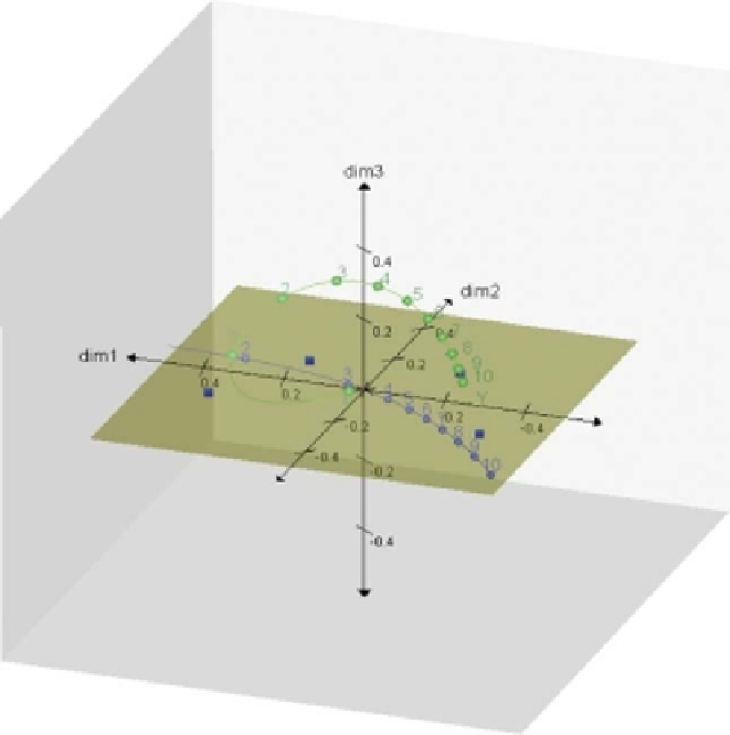
Figure 5.14
Calibrated normal projection prediction biplot axis for original variable
Y
.
projection of O onto the intersection space, we first calculate the orthogonal projection,
S, of the point R onto the line
l
∗
(µ)
,where
l
∗
(µ)
has been translated vertically by
−
t
(µ)/
l
2
(µ)
units to pass through the origin. The coordinates of the point R are given
by
(
0,
−
t
(µ)/
l
2
(µ))
and the line
l
∗
(µ)
is generated by the vector
(
l
2
(µ)
,
−
l
1
(µ))
,sothat
the projection S is given by
(
l
1
(µ)
t
(µ)
,
−
l
1
(µ)
t
(µ)/
l
2
(µ))
. The point P representing the
marker
µ
on the
k
th prediction biplot trajectory is given by
l
1
(µ)
t
(µ)
,
0,
=
l
1
(µ)
t
(µ)
,
l
2
(µ)
t
(µ)
.
l
1
(µ)
(µ)
l
2
(µ)
t
(µ)
l
2
(µ)
t
+
−
This is illustrated for the intersection spaces where
2, 3 and 4 for the original variable
Y
in Figure 5.17 in
R
with three dimensions and in Figure 5.18 in
L
with two
dimensions. If we let
µ
=
vary continuously from 0 to 10, a series of intersection spaces
is formed and, connecting the projections of O onto each of these, produces the circular
prediction biplot trajectory as shown in Figure 5.19.
To predict the value of original variable
Y
for the point P in the approximation space,
a circle is constructed with OP as diameter. The diameter OP subtends a right angle at
µ