Information Technology Reference
In-Depth Information
The first summation in (5.13) gives the vector sum for the markers
x
1
,
x
2
,
...
,
x
p
of
the pseudo-samples, while the second summation gives the interpolant of the mean
(
0, 0,
...
,0
)
, that is, the point of concurrency of the trajectories.
5.4.2 Prediction biplot axes
To construct prediction biplot axes in
L
for our example, the process follows similar
principles to those described for the linear PCA and CVA biplots in Sections 3.2.3
and 4.4.2, respectively. To predict the marker
µ
on the
k
th biplot axis, a plane
N
is
constructed at the point corresponding to
e
k
. The plane
N
is normal to the embedded
Cartesian axes in
R
+
. All points in this plane predict the value
µ
for the
k
th variable.
This plane,
N
, intersects the (in general)
r
-dimensional approximation space,
L
,in
an (
r
µ
−
1)-dimensional linear subspace
L
∩
N
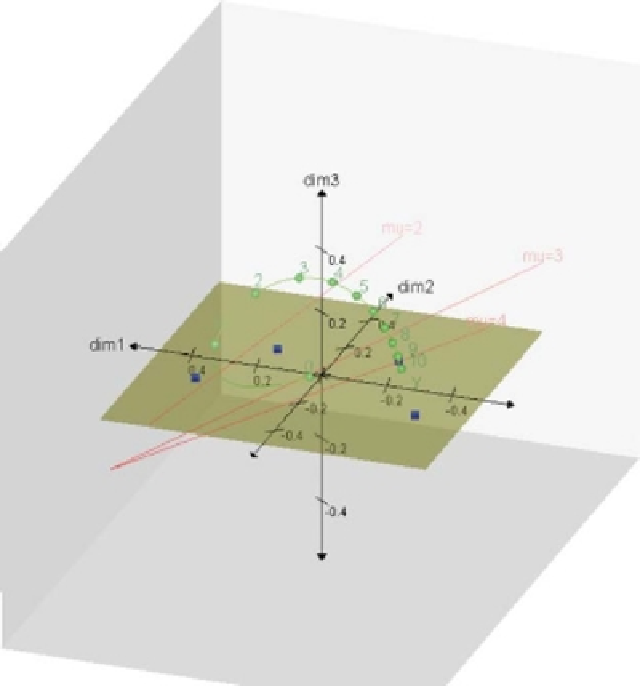
. Since embedding the marker
µ
e
k
in
Figure 5.12
Intersection spaces
L
∩
N
for the original variable
Y
at the points
µ
=
2, 3, 4.