Information Technology Reference
In-Depth Information
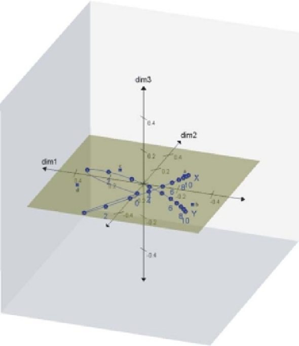
Figure 5.11
Representation of sample points in biplot space together with the nonlinear
interpolation biplot axes projected onto the two-dimensional biplot space.
It follows from (5.11) that for a new sample
x
=
k
=
1
x
k
e
k
we have
p
p
p
d
n
+
1,
i
(
x
)
=
d
2
d
n
+
1,
i
(
x
k
)
−
(
p
−
1
)
d
2
(
x
ik
,
x
k
)
=
(
x
ih
,0
)
k
=
1
k
=
1
h
=
1
so that
p
p
1
2
d
2
d
n
+
1
(
x
)
=
d
n
+
1
(
x
k
)
−
(
p
−
1
)
1
{−
(
x
ih
,0
)
}
.
(5.12)
k
=
h
=
1
Substituting (5.12) into (5.9) leads to the expression for vector-sum interpolation:
=
−
1
Y
p
n
D1
p
−
)
−
1
2
d
2
1
y
d
n
+
1
(
x
k
)
−
(
p
−
1
)
(
x
ih
,0
k
=
1
h
=
1
p
p
n
D1
d
n
+
1
(
n
D1
−
(
−
)
−
=
−
1
Y
1
1
2
d
2
1
x
k
)
−
p
−
1
)
(
x
ih
,0
.
(5.13)
h
=
1
k
=
1