Information Technology Reference
In-Depth Information
back-projection. The PCA prediction axes, so obtained, would allow us only to predict
the values of the canonical variables, whereas we would like to predict values of the
observed measurement scales of
X
. The key is that a coordinate
y
plotted as a canonical
sample point is obtained from an observed sample
x
by
y
=
x
M
and therefore
x
=
y
M
−
1
.
This shows that the values of
x
may be predicted from the inner products of the
sample point
y
in canonical space with the rows of
M
−
1
, which therefore represent
the directions of axes for the original variables. These axes are not orthogonal but
nevertheless the back-projection mechanism for PCA remains valid. In particular, the
directions of the prediction axes in the
r
-dimensional approximation are obtained from
JM
−
1
.The
k
th of these axes has direction
JM
−
1
e
k
. It follows that in contrast to PCA
where only the calibrations on predictive axes differ from those of interpolative axes,
for CVA the directions
JM
−
1
e
k
of prediction axes also differ from the directions
e
k
MJ
of the corresponding interpolative axes.
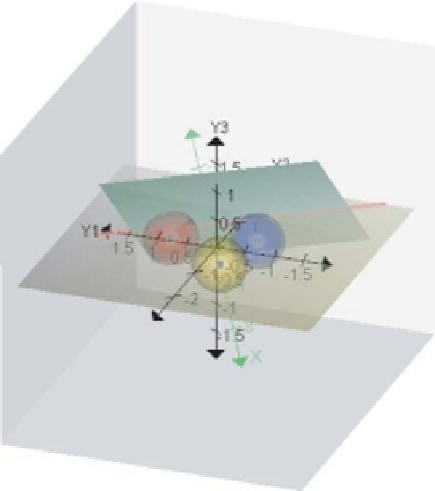
It remains only to calibrate the prediction axes. We construct a plane
N
orthogonal
to the
k
th embedded original axis as illustrated for
X
through the point
4. This
is illustrated in Figure 4.9. Any point on the plane
N
is of the form (4.9) and predicts
the value
µ
for the
k
th original axis, therefore
y
M
−
1
e
k
=
µ
. This defines the equation
for the plane
N
and the intersection
L
∩
N
lies in
L
with equation
z
JM
−
1
e
k
µ
=−
=
µ
.
β
k
.To
facilitate orthogonal projection onto the biplot axes, we choose
β
k
to be orthogonal to
z
JM
−
1
e
k
We therefore have the biplot axis
β
k
in
L
with the marker
µ
a point on
=
µ
and therefore of the form
τ
e
k
(
M
−
1
)
J
for -
∞
<τ<
∞
.Topredictthe
Figure 4.9
Construction of prediction biplot axes with the plane
N
orthogonal to
original variable
X
.