Information Technology Reference
In-Depth Information
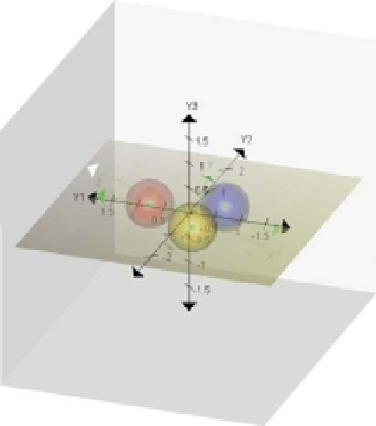
Figure 4.8
Biplot space aligned with the first two dimensions of the display.
4.4 CVA biplot axes
4.4.1 Biplot axes for interpolation
The transformation matrix
L
found in the first step of the two-step CVA procedure
transforms the original space to the canonical space. The second step, as we have seen,
is just an ordinary PCA in the canonical space, thus leading to the principal axes
Y
=
LV
in the canonical space. Therefore, interpolative biplot axes can be constructed
precisely as described in Section 3.2.2 for PCA biplots by simply doing first the same
transformation on the original unit points
e
k
(
k
=
1, 2,
...
,
p
)
of the Cartesian axes of
X
to
obtain
e
k
L
. This is valid because the unit points have the same form as the sample values
and, indeed, are themselves putative data observations. Since the full transformation is
defined by
y
=
x
LV
x
M
, and transformation to the
r
-dimensional biplot space by
z
=
x
MJ
,
=
(4.9)
the direction and calibration of the marker
µ
on the
k
th interpolation biplot axis is
e
k
MJ
,where
µ
µ
∈
(
−∞
,
∞
)
. Thus, unit markers for all the interpolation biplot axes
are given by the rows of
MJ
.
4.4.2 Biplot axes for prediction
We know that the direction of a predictive biplot axis in PCA is given by the orthogonal
projection of the full axis onto the biplot space, with appropriate markers obtained by