Canonical variate analysis biplots - Understanding Biplots - page 159

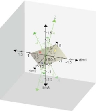
(a) (b)
Figure 4.7 (a) Canonical means after the step I transformation by the matrix L .
(b) PCA now implies fitting the least-squares plane of best fit to the canonical means in
step II.
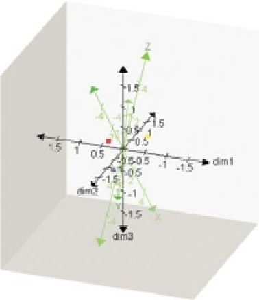
the biplot axes from Figure 3.9 which is equivalent to Figure 4.7(b). However, since
rotations do not have any effect on the distances, we can rotate Figure 4.7(b) to have the
two-dimensional PCA plane aligned with the first two dimensions. This is illustrated in
Figure 4.8.
Figure 4.8 gives the final representation in the full canonical space. Any sample point
x can be represented in the two-dimensional CVA biplot with the transformation x LV J
or x MJ which amounts to orthogonal projection onto the plane shown in Figure 4.8.
The projection of the spheres amounts to their intersection with the above plane. Since
there are only three classes in this example, the maximum number of dimensions needed
to separate the three class means is two and then the two-dimensional CVA biplot is an
exact representation of the three optimally separated class means. The three class means
lie in the plane, even without orthogonal projection. In this case classification regions are
just the nearest-neighbour regions for the means in the plane shown in Figure 4.8. With
more than three means, a representation in two dimensions is not exact and the means
are not contained in two dimensions. Then, the neighbour regions in two dimensions are
given by those points that are nearest the true multidimensional means rather than to
their projections (see (4.8)).
Notice that the axes representing the original variables X , Y and Z are embedded
via a simple linear transformation into this space. In the next chapter we will see how to
embed axes with more complex nonlinear transformations, but the underlying principle
is the same.