Principal component analysis biplots - Understanding Biplots - page 105

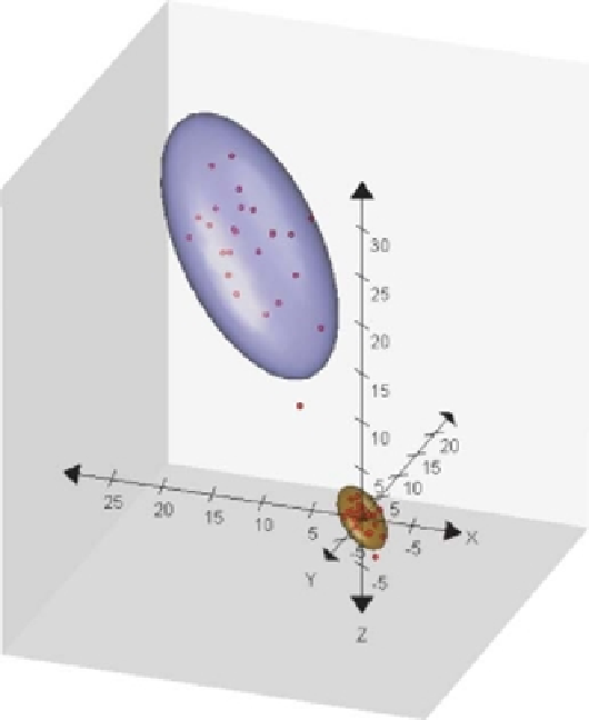
Figure 3.26 Three-dimensional display of the unscaled data of Table 3.3 (blue ellipse)
and the scaled data given in Table 3.18 (brown ellipse).
with time, so generating a strong unidimensional trend. Pay load factor is an exception,
with some very small values in later years, possibly to be identified with aircraft designed
for surveillance rather than carrying capacity.
What happens when the data are scaled? To illustrate the effect of scaling, the data of
Table 3.3 have been scaled to have mean zero and unit standard deviation (see Table 3.18).
Compare Figure 3.3 with Figure 3.26. There was no change in the correlations in the
data, resulting in an ellipsoid with the same orientation as that of Figure 3.3. However,
since the variance for each of the three Cartesian axes is equal, the ellipsoid has a more
spherical shape. A new plane of best fit is obtained for this data set (minimizing the
distances between the samples and their projections onto the plane) and a new projection
matrix results in new biplot axes. Many other scalings can be performed on the data,
each resulting in a different PCA biplot representation. The benefit of scaling the data
before constructing the biplot depends on the practical interpretation resulting from that
specific scaling.
The effect of scaling the Table 3.3 data on the biplot is minimal as can be judged by
comparing Figures 3.17 and 3.27. Only slight changes in the relative position of samples,
for example 9 and 11 (just above 23 in Figure 3.17), can be observed.