Environmental Engineering Reference
In-Depth Information
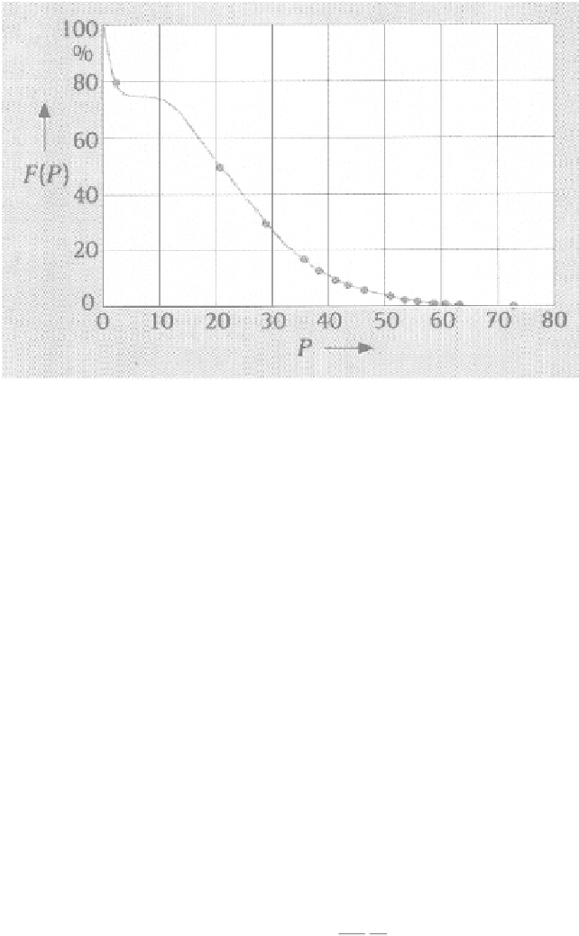
Fig. 7.14
Example from an arc furnace of a cumulative flicker power curve to determine
P
lt
(length exaggerated in the Figure) is
ϕ
f
. In the example, the angle sum is approxi-
80
◦
. Hence the projection of
Z
k
Δ
mately (
I
on
U
V
indicating the voltage
variation is rather small. Note that
c
decreases with the cosine of the angle sum and
can theoretically become zero. Regulations, however, prescribe to limit and set the
cos-value = 0
,
1if
ψ
k
+
ϕ
f
)
≈
<
0
,
1.
Flicker coefficients vary with ratings and are generally larger for turbines with
stall control than with pitch control. For a system where
c
is known, the long term
flicker strength is calculated from equation (7.9) rearranged:
|
cos(
ψ
kV
+
ϕ
f
)
|
S
k
cos
(
ϕ
f
)
S
n
P
lt
=
c
·
ψ
kV
+
Noting that for a given WES the flicker coefficient is a function of the short-
circuit impedance phase angle, the manufacturers are requested to declare
c
for se-
lected values of the short-circuit impedance phase angle:
S
k
S
n
c
(
ψ
k
)=
P
lt
(
ψ
k
)
·
(7.10)
Further, a grid-dependent switching current factor is defined which describes the
influence of the system current on voltage variations:
ψ
k
)=
Δ
U
U
S
k
S
n
k
i
ψ
(
(7.11)
In Table 7.2 characteristic values for selected systems (the same as in Table 5.1)
are collated which are relevant for flicker and switching properties; also part-load
power factors and permissible peak power values are given.
Search WWH ::

Custom Search