Environmental Engineering Reference
In-Depth Information
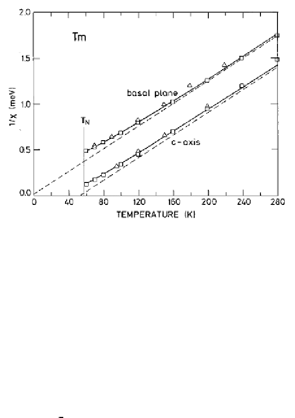
Fig. 2.1.
The inverse susceptibility, in atomic units, in Tm above
T
N
.
The full lines depict the results of a mean-field calculation and the dashed
lines are extrapolations of the high-temperature limit. Experimental val-
ues are also shown. The MF theory predicts a deviation from the high-
temperature expression as the ordering temperature is approached from
above, because of crystal-field anisotropy effects.
ments are the bulk values at zero wave-vector. The straight lines found
at high temperatures for the inverse-susceptibility components 1
/χ
αα
(
0
)
versus temperature may be extrapolated to lower values, as illustrated in
Fig. 2.1. The values at which these lines cross the temperature axis are
the
paramagnetic Curie temperatures
θ
, determined respectively
when the field is parallel and perpendicular to the
c
-axis (
ζ
-axis). The
high-temperature expansion then predicts these temperatures to be
and
θ
⊥
=
3
−
5
−
2
)(
J
+
2
)
B
2
,
k
B
θ
J
(
J
+1)
J
(
0
)
(
J
(2
.
1
.
15
a
)
and
=
3
(
0
)+
5
−
2
)(
J
+
2
)
B
2
.
k
B
θ
J
(
J
+1)
J
(
J
(2
.
1
.
15
b
)
⊥
Hence the paramagnetic Curie temperatures are determined by the
lowest-rank interactions in the Hamiltonian, i.e. those terms for which
l
+
l
= 2. The difference between the two temperatures depends only on
B
2
, because of the assumption that the two-ion coupling is an
isotropic


Search WWH ::

Custom Search