Agriculture Reference
In-Depth Information
plant can sustain a fixed number of lesions and the spore production rate depends on
the number of infectious lesions. Spores are dispersed from an infected plant and
deposited on other plants according to a 'primary deposition function',
PDF
, which
is a function of the distance between the source plant and the receptor plant. The
model can be formulated in terms of the rate of production of new lesions and the
rate of death of old lesions for all the plants. For a given plant, the rate of production
of active lesions depends on the existing number of lesions (active and passive) and
on the previous rate of spore deposition from all other plants at time
T
l
(effect of
latent period). The rate of production of passive lesions depends on the rate of
production of active lesions at time
T
p
. The model then calculates the development
of lesions with time on each individual plant from some initial infection conditions,
for example a single infected plant (Fig. 6.1). This type of model can be formulated
as continuous differential equations, as discrete time difference equations or as
stochastic functions (Shaw, 1994, 1995, 1996; Xu and Ridout 1996, 1998). For
stochastic solutions, the functions defining lesion production, spore production and
spore dispersal are formulated as probabilities. Stochastic simulation models are
equivalent to Lagrangian stochastic models used in particle dispersal modelling in
that they use many simulations of individual dispersal events to accumulate
information on the spatial and temporal dynamics of the epidemic. Disease
simulation models differ in the method by which the various steps in the disease
cycle are formulated but each model includes the equivalent of a 'primary
deposition' function.
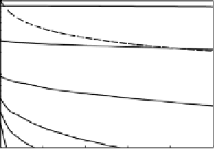
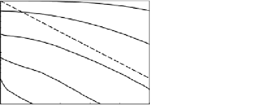
Figure 6.1. Simulated disease progress curves. Output of a simple one dimensional disease
progress model illustrating the difference between exponential primary dispersal function
(PDF)
(left hand graph) and a power law
PDF
(long tailed distribution) (right hand graph).
Both models had the same infection and sporulation characteristics and latent and
sporulation periods. The
PDFs
are shown as dashed lines. The exponent of the power law
PDF
was chosen so that it had a similar slope to the exponential
PDF
when plotted over three
exponential half distances. Initial disease intensity at the focus was set at 1% area infected.
Distance is plotted in units of exponential half distance (distance/ half distance). The numbers
associated with each curve are latent periods from the start of the epidemic. Exponential
PDFs
result in a 'travelling disease wave'. Long-tailed
PDFs
give a dispersive wave front (the
gradient flattens with time).