Biology Reference
In-Depth Information
X
2
PC2
PC1
S
2
PC2
S
1
S
1
PC1
S
2
X
1
X
1
(A)
(B)
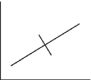
FIGURE 6.3
Graphical interpretation of PC scores. (A) The star is the location of an individual in the sample.
Perpendiculars from the star to PCs indicate the location of the star with respect to those axes. The distances of
points
S
1
and
S
2
from the sample centroid (intersection of PC1 and PC2) are the scores of the star on PC1 and
PC2. (B) The figure in part A has been rotated so that PCs are aligned with the edges of the page. The PCs will
now be used as the reference axes of a new coordinate system; the scores on these axes are the location of the
individual in the new system. The relationships of the PC axes to the original axes has not changed, nor has the
position of the star relative to either set of axes.
In effect, we are rotating and translating the ellipse into a more convenient orientation so
we can use the PCs as the basis for a new coordinate system (
Figure 6.3B
). The PCs are the
axes of that system. All this does is allow us to view the data from a different perspective;
the positions of the data points relative to each other have not changed.
As suggested by
Figure 6.4
, we could compute an individual's score on a PC from the
values of the original variables that were observed for that individual and the cosines of
the angles between the original variables and the PCs. In our simple two-dimensional
case, the new scores,
Y
, could be calculated as:
Y
1
5
A
1
X
1
1
A
2
X
2
(6.1)
where
A
1
and
A
2
are the cosines of the angles
α
2
and the values of individuals on
X
1
and
X
2
are the differences between them and the mean, not the observed values of
those variables.
It is important to bear in mind for our algebraic discussion that
Equation 6.1
represents
a straight line in a two-dimensional space. Later we will see equations that are expansions
of this general form and represent straight lines in spaces of higher dimensionality. So, in
case the form of
Equation 6.1
is unfamiliar, the next few equations illustrate the simple
conversion of this equation into a more familiar form. First, we rearrange the terms to
solve for
X
2
:
α
1
and
Y
1
2
A
1
X
1
5
A
2
X
2
(6.2)