Biology Reference
In-Depth Information
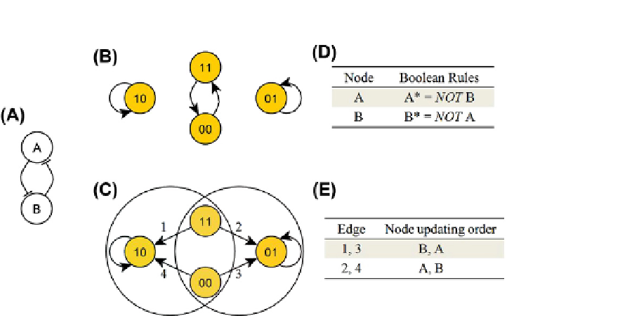
FIGURE 10.3
Ilustration of the basins of attraction of a system under different updating schemes. The system is composed of two mutually
inhibiting nodes A and B (A). The Boolean functions are given in table (D). (B) and (C) show the state transition graphs of the system under
synchronous update (B), and random order asynchronous update (C). The 2-digit vectors inside the circles represent the states of node A and B from
left to right. In the case of random order update (C) the correspondence between the order in which A and B are updated and the particular state
transitions, indicated by edge labels, is given in table (E). E.g., starting from an initial state of 11, if A is updated first and B is updated second, state 11
will evolve into state 01. The two unlabeled self-loops on states 01 and 10 in both (B) and (C) indicate that if the system is currently in one of those
states, the future state will be the same as the current state, regardless of the manner of update, thus these are fixed points of the system. Under
synchronous update (B), the system has 3 attractors: the two fixed points 01 and 10, and a cyclic attractor. Only the fixed points are preserved under
asynchronous update (C). In (C), the states 11, 00, 10 form the basin of attraction of 10, and states 11, 00, 01 form the basin of attraction of 01. The
states11and00belongtobothbasinsofattraction.
whole system correspond to known biological events,
such as certain phases of the cell cycle
[8,47]
, apoptosis
and cell differentiation
[48]
, and hence the first focus,
identifying attractors of
the general asynchronous scheme equals the total number
of nodes in the system. The system state will traverse all
states in the attractor shown in
Figure 10.5
(B)), following
the outgoing edges with a certain calculable probability.
For both types of update, the average state level of the node
Output (the last digit) in the attractor is 0.5. This could be
interpreted as a 50% up time of a certain system activity.
The critical network motif
[49]
of the original
network is the negative feedback on node A. It is the
negative feedback, coupled with the Boolean AND rule
for node A, that generates the oscillatory behavior of the
system.
The next example network (
Figure 10.6
) differs from the
previous one (
Figure 10.4
) in that it contains one more edge
from B to the Output, and the state of the Output is deter-
mined by A and B independently, in a Boolean OR relation.
We already know that the negative feedback on node Awill
generate an oscillatory behavior for itself as well as for node
B, but does the new edge help improve the activation of the
Output? The answer is yes. Under both updating schemes
the average state level of the Output is ~0.75. If the Boolean
relationship between A and B in the Output function is
changed to AND, the Output level drops to ~0.25. It is
indeed reasonable that a more stringent condition for acti-
vation will reduce the average Output level. Under
synchronous update, the Output (and also the system) will
have period-4 oscillations. In the state transition graphs of
the system (
Figure 10.7
), (A) corresponds to Output*
the whole system,
is most
relevant.
The fixed points of a Boolean network model can be
determined in several ways. One can analytically solve the
Boolean equations. Since the system being in the steady
state means that the state vector remains time-invariant, the
future state of any node will be the same as its current state.
Thus, the time-dependent features (indices or asterisks) of
the Boolean equations can be removed and the set of
resulting time-independent equations can readily be solved.
One can also do repeated dynamic simulations of the
system, updating the nodes' states according to their
Boolean rules. One can also draw useful conclusions from
the existence of particular interaction patterns (called
'network motifs')
[49]
, such as feedforward or feedback
loops (as first suggested by Thomas,
[50]
). Consider the
following examples.
In the example of
Figure 10.4
, the system (hence also
the Output) has a single attractor for any update method.
For synchronous update, the attractor is a cycle of period 4
(
Figure 10.5
(A)). Under general asynchronous updating the
attractor spans the whole state space. Every state in the
latter attractor has multiple edges, both incoming and
outgoing (
Figure 10.5
(B)). This is because a state can have
different successor states if a different node is updated. The
maximum number of possible outcomes from a state under
¼
A
OR B, and (B) to Output*
¼
A AND B.