Civil Engineering Reference
In-Depth Information
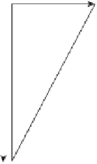
U
top
∗
y
g
V
slip
x
L
s
> 0
16.8
Hydrodynamic slip fl ow profi le characterized by slip length
L
s
(adapted from Choi
et al.
, 2011).
differs from that of the solid, we usually say the surface imposes a slip
boundary condition as depicted in Fig. 16.8 (Choi
et al.
, 2011). The slip
boundary condition helps us describe non-continuum behaviour of water
transport inside the CNT in the framework of continuum dynamics. For
example, slip length,
L
s
, may serve as a good indicator for the molecular
interaction between water molecules and CNT via provision of information
about the degree of departure the transport innately has from the hydro-
dynamic Hagen-Poiseuille fl ow. Also, the slip length indicator can compare
with results of molecular dynamics (MD) simulations often used for the
exact prediction of water fl ow under the CNT nanoconfi nement.
Slip length,
L
s
, is convenient to explain the hydrodynamic boundary
condition at the interface of fl uid and wall, which is defi ned according to
the Navier boundary condition:
∂
∂
v
n
t
L
=
v
−
v
[16.2]
s
t,wall
wall
′
wall
where
n
and
t
denote normal and tangential directions of the wall,
v
t
is the
velocity of a fl uid tangential to the wall, and
v
wall
is the velocity of the wall.
v
t,wall
v
wall
is denoted as a slip velocity.
The solutions for the velocity and the corresponding volume fl ow rate in
the fl ow direction,
z
, with respect to the distance from the centre,
r
, have a
parabolic profi le given by:
−
2
2
dp
dz
Rr
R
⎛
⎜
2
L
R
⎞
⎟
s
U
=−
1
−
+
[16.3]
s
2
4
μ
dp
dz
π
R
4
Q
=−
[16.4]
Hagen
−
Poiseuille
8
μ
4
L
R
⎛
⎝
⎞
⎠
s
QQ
=
1
+
[16.5]
s
Hagen
−
Poiseuille


Search WWH ::

Custom Search