Wind turbine acoustics - Wind Power Generation and Wind Turbine Design - page 178

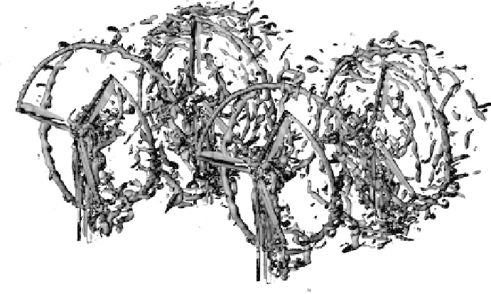
Figure 19: Large-scale vortices around four wind turbines visualized by the l 2
method.

however, this approach is computationally costly, leading to the development of
several noise propagation models during the years. A review of the noise propaga-
tion models are presented in [4].

6.4.1 Spherical spreading model
The simplest propagation model is to assume spherical spreading. This implies
that the sources are considered point sources and all the parameters enumerated
in Section 4.2 are neglected, except the distance to the observer. According to the
spherical propagation model the sound pressure level decreases with 6 dB for a
doubling of the source − observer distance.

6.4.2 VDI 2714
One of the most simple and widely used models is the VDI 2714 method, where the
sound pressure level at a receiver is given by the following empirical formula [4]:

L L DKLLLLLL = ++−−−−−−

(38 )

p w d a g v b s

where D accounts for the source directivity, K is a correction for the refl ec-
tion of sound due to the presence of vertical walls ( K = 0 dB for sound sources
located in the free fi eld, K = 3 dB above the ground, and K = 6 dB or K = 9
dB when two or three perpendicular surfaces are present, respectively). L d = 10
log 10 (4 p r 2 ) accounts for the infl uence of the source

observer distance. The air
absorption effect is represented by L a = a r . The ground effects are modeled as
g

−

where h m is the average of the source and
observer heights. The last three terms in eqn (38) account for the infl uence of the
vegetation, buildings and screens, respectively.

L =− [4.8 (2 h / )(17 r + (300 / ))] r

m