Aerodynamics and aeroelastics of wind turbines - Wind Power Generation and Wind Turbine Design - page 101

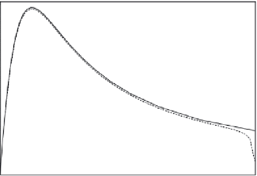
Optimum Blade Shape C-L = 1 B = 3

0.2

Glauert
De Vries

0.15

0.1

0.05

0

0 0.2 0.4 0.6 0.8 1

r/R

Figure 13 : Optimum shape of a blade.

3 Numerical CFD methods applied to wind turbine fl ow

As a complement to analytical theories and experiments, CFD provides a third
approach in developing applied methods. In its purest form, only the differential
equations of Navier and Stokes (NS):

∇= · v ,

(34)

Dv

( 35 )

r =−∇+Δ= f p v m 0

Dt

together with suitable boundary conditions and a description of the blade geom-
etry is used. Unfortunately this ambitious goal cannot be reached at the pres-
ent time. The main obstacle is the emergence of turbulence at higher Reynolds
number (RN):

vL

( 36 )

Re =

n

calculated from kinematic viscosity ( v = 1.5 - 10 -5 m 2 /s -1 for air) and a typical
length L and a typical velocity v . Present wind turbines have a RN of several mil-
lion based on blade chord. Only Direct Numerical Simulation (DNS) solves the
(NS) without any further modeling. At the present time (2009), only airfoil calcu-
lations up to RN of a few thousands have been carried out at the price of months