Add Motion with JavaFX Animation - JavaFX: Developing Rich Internet Applications - page 192

x => 1000 tween Interpolator.SPLINE(x1, y1, x2, y2)

When the cubic spline is plotted, the slope of the plot defines the acceleration at
that point. As the slope approaches vertical, the acceleration increases; when the
slope of the plot approaches horizontal, the motion decelerates. If the slope of
the line at a point is 1.0, the interpolation is moving at a constant rate of change.
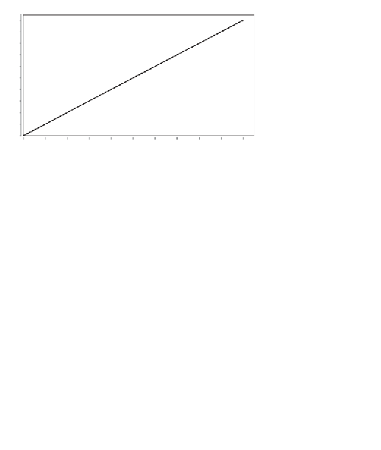
Figure 7.2 shows the spline plot equivalent to the LINEAR built-in interpolator.
This reflects a constant rate of change, as the slope for the entire line is 1.0.

Linear

1.0

0.9

0.8

0.7

0.6

0.5

0.4

0.3

0.2

0.1

0.0

0.0 0.1 0.2 0.3 0.4 0.5 0.6 0.7 0.8 0.9 1.0

Time

Figure 7.2 Linear - Cubic Spline for Linear Interpolation

The control points for the spline are (0.25, 0.25) and (0.75, 0.75), which results
in a straight line with a slope of 1. This represents a constant speed from the start
of the time period to the end.

x => 1000 tween Interpolator.SPLINE(0.25, 0.25, 0.75, 0.75)

Figure 7.3 represents the plot for an ease both interpolation. Here the control
points are (0.2, 0.0) and (0.8, 1.0).

x => 1000 tween Interpolator.SPLINE(0.2, 0.0, 0.8, 1.0)

Notice that the slope is flat near the beginning and end of the plot. So the motion
will start slow and accelerate for the first 20% of the time period, stay at a con-
stant speed until the last 20% of the time period, when it will decelerate.

By using the Interpolator SPLINE() function, you can easily create unique inter-
polation behavior. However, for performance reasons, stick to the predefined
interpolators if that is what you want.